Part 1 · vLLM internals
Inside vLLM: Following One Request from the API to GPU Execution
This English edition is adapted from the published Chinese article on Zhihu. It preserves the source-code references, experimental boundaries, and reproducible artifacts while adapting the structure for an international engineering audience.
This article follows one offline inference request through vLLM V1: from
LLM.generate() and inter-process communication to scheduling, input
flattening, GPU model execution, paged KV-cache access, sampling, and resource
reclamation. The goal is to answer one concrete question: what happens behind
the call to llm.generate() before the completed result reaches the caller?
The discussion assumes familiarity with Transformer inference, including prefill, decode, KV caching, and autoregressive generation. It focuses on how those concepts appear in vLLM source code rather than reteaching the model architecture.
Version scope. The source references were verified against vLLM 0.22.0; this edition was checked on September 3, 2026. vLLM evolves quickly, so some filenames and call boundaries will move. The long-lived ideas—continuous batching, token budgets, paged KV allocation, and the separation between scheduling and execution—are the real subject of the article.
Why Read the Source Instead of Another API Guide?
Many introductions stop at the useful analogy that PagedAttention manages the KV cache much like virtual memory manages pages. The analogy does not tell us how a request is admitted, how variable-length requests become a flat token batch, or what the page table looks like at the kernel boundary.
The answers are in the source. This article follows vLLM 0.22’s V1 execution path from the public entry point to the CUDA boundary. It is a source-code walkthrough, not an API tutorial.
Start with a System Map
Start with the process boundary and the engine loop. In vLLM V1, EngineCore runs continuously in a child process. Requests enter and leave the active set between steps; the caller does not drive GPU execution one token at a time.
One detail shapes the entire path: in this configuration, vLLM 0.22 separates the caller-facing engine from EngineCore with a process boundary.
REQUEST SUBMISSION · main process -> EngineCore child

Caller
  └─ LLM.generate(prompts)
       └─ LLMEngine.add_request()
            └─ EngineCoreClient
                 └─ IPC input queue ──────────────▶ scheduler.add_request()

CONTINUOUS ENGINE LOOP · EngineCore child

run_busy_loop()
  ├─ receive newly submitted requests
  └─ repeat EngineCore.step()
       1. scheduler.schedule()
          └─ spend token / KV-cache budgets -> SchedulerOutput
       2. model_executor.execute_model()
          └─ GPU forward pass and sampling -> sampled tokens
       3. scheduler.update_from_output()
          ├─ update request state and release finished KV blocks
          └─ EngineCoreOutputs ───────────────▶ IPC output queue

RESULT CONSUMPTION · EngineCore child -> main process

IPC output queue
  └─ LLMEngine.step() / get_output()
       └─ detokenize and assemble RequestOutput
            └─ return completed results to LLM.generate() and the caller
This map establishes three boundaries used throughout the article.
First, the main process consumes results; EngineCore produces them. Calling
LLMEngine.step() does not tell the GPU to perform one step. It retrieves
already-produced output through get_output(), then detokenizes and assembles
the user-facing result. Scheduling and model execution advance independently
inside EngineCore’s busy loop.
Second, EngineCore.step() has three core stages: scheduling, execution, and
state update. The rest of the article expands those stages one at a time.
Third, this loop implements continuous batching. The request set changes from
one step to the next: stage 3 removes completed requests and releases their
resources, while the next call to schedule() can admit waiting work. The GPU
therefore does not have to wait for one fixed batch to finish before admitting
another request.
The Path We Will Follow
The rest of the article expands that loop into six parts:
- Entry: how
LLMandLLMEnginesubmit work to EngineCore. - Scheduling: how
schedule()spends token and KV-cache budgets. - Input preparation: how variable-length requests become flat tensors.
- Model execution: how metadata reaches attention inside the forward pass.
- PagedAttention: how the write and read paths address KV-cache blocks.
- Output: how logits become tokens and completed requests release resources.
Each part keeps only the code needed to connect one boundary to the next.
Part 1: The Entry Point Behind generate()
Start with the public interface:
from vllm import LLM, SamplingParams

llm = LLM(model="facebook/opt-125m")
outputs = llm.generate(["Once upon a time"], SamplingParams(max_tokens=50))
Those two lines initialize the entire engine stack. Start with the LLM class.
LLM Is a Thin Wrapper
In entrypoints/llm.py, LLM delegates engine construction to one factory
call:
# entrypoints/llm.py
self.llm_engine = LLMEngine.from_engine_args(
    engine_args=engine_args,
    usage_context=UsageContext.LLM_CLASS,
)
LLM packages model, dtype, and other configuration into EngineArgs, then
uses the factory method to create LLMEngine. It is the public facade;
LLMEngine owns the request-processing path followed below.
generate() returns a list[RequestOutput], one complete result per request.
The generated text is available as output.outputs[0].text.
The distinction is useful throughout the article: LLM is the facade, while
LLMEngine connects that facade to EngineCore.
At Its Core, generate() Is a Loop
The internal logic of generate, after stripping away the details, is as follows:
# Conceptual skeleton
for prompt in prompts:
    self.llm_engine.add_request(prompt, ...)   # 1. Register the request with the engine

outputs = []
while self.llm_engine.has_unfinished_requests():  # 2. While any request is unfinished
    step_outputs = self.llm_engine.step()         #    advance the engine by one step
    for out in step_outputs:
        if out.finished:
            outputs.append(out)
return outputs                                     # 3. Return after collecting every result
This while ... step() loop continues until every submitted request is
finished. Unlike a hand-written for _ in range(max_tokens) loop over one
sequence, it tracks a set of requests whose lengths and completion times differ.
step() Does Not Submit the Request
The name step() can suggest a synchronous “submit, execute, return” call.
The implementation does something different:
# v1/engine/llm_engine.py (simplified)
def step(self):
    # 1) Fetch outputs already produced by EngineCore
    outputs = self.engine_core.get_output()

    # 2) Decode tokens and evaluate stopping conditions
    processed = self.output_processor.process_outputs(outputs.outputs, ...)

    # 3) Handle requests terminated by a stop string
    self.engine_core.abort_requests(processed.reqs_to_abort)

    # 4) Record statistics
    ...

    return processed.request_outputs
step() never submits a request or directly drives model execution. It calls
get_output() to consume results. Submission already happened in
add_request(); the actual computation runs independently elsewhere.
This description assumes the default multiprocess V1 configuration. If
VLLM_ENABLE_V1_MULTIPROCESSING=0 is set for debugging, the in-process client
drives EngineCore from get_output() and the child-process producer/consumer
boundary collapses. The scheduling, execution, and update stages discussed
below still apply, but they no longer run in a separate EngineCore process.
This producer-consumer split is asynchronous across the process boundary. In configurations that enable asynchronous scheduling, the startup log also states:
INFO ... Asynchronous scheduling is enabled.
That “elsewhere” is a separate child process. A running server prints a prefix
such as (EngineCore pid=8884) in its logs: this is the EngineCore process
that performs scheduling and model execution.
The main process (LLMEngine) is the consumer: get_output() receives results,
decodes them, and returns them to the caller. The child process (EngineCore)
is the producer: its busy loop schedules requests, runs the model, produces
tokens, and writes results to an IPC queue.
This lets host-side output processing overlap EngineCore execution. In an online server, request tokenization and admission can also proceed independently of an already-running GPU step. The IPC queues separate those execution timelines.
What This Part Established
LLMis the facade;LLMEngineis the engine entry point.- At the heart of
generateis thewhile has_unfinished_requests(): step()loop. LLMEngine.step()consumes and decodes output; the separateEngineCoreprocess performs scheduling and execution asynchronously.- IPC decouples production in the child process from consumption in the main process, allowing CPU work to overlap GPU execution.
Next we cross the IPC boundary and enter EngineCore, whose busy loop has three
core stages: schedule, execute, and update.
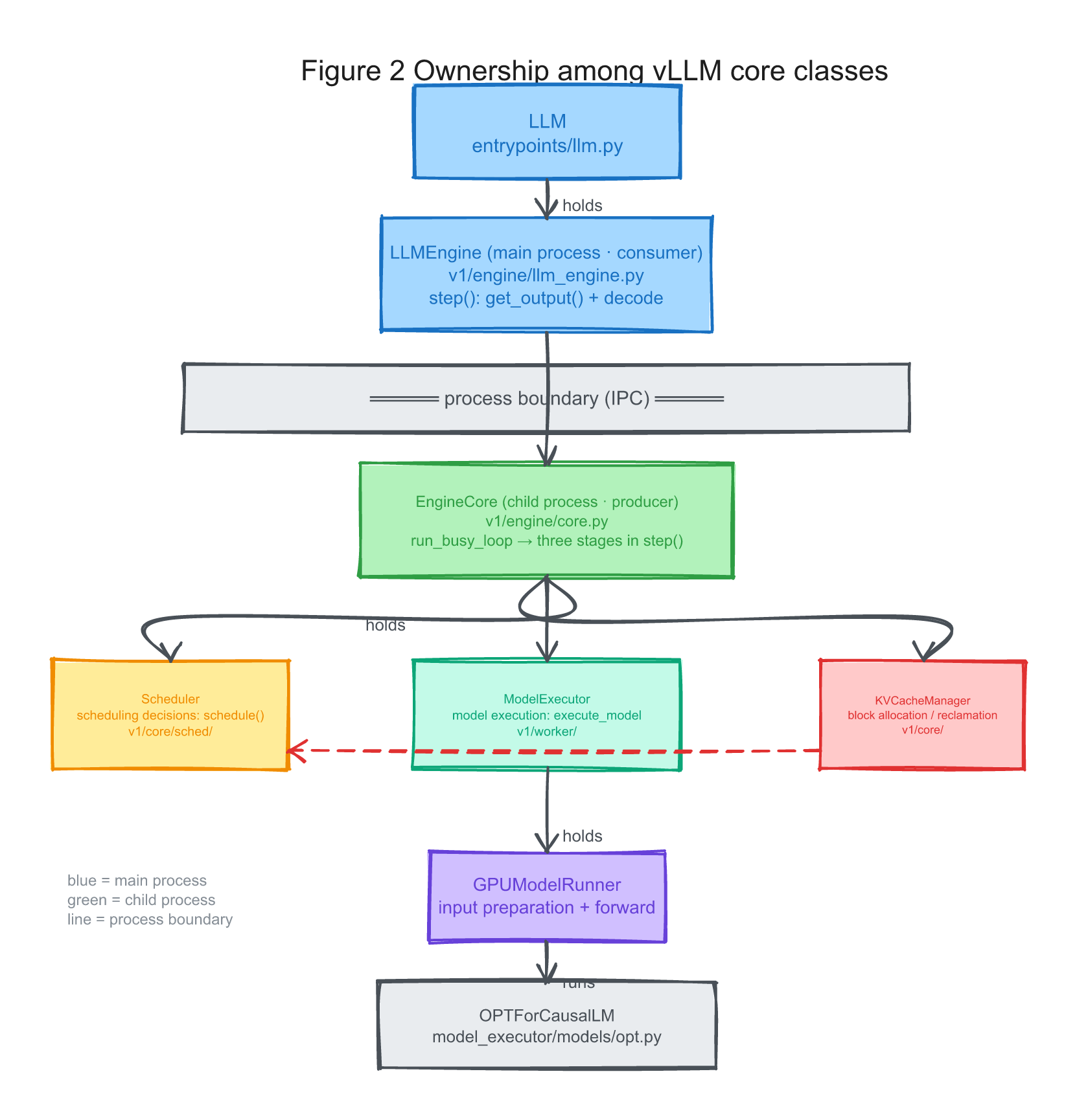
Figure: ownership among vLLM’s core classes.
LLMownsLLMEngine, which communicates withEngineCore;EngineCorein turn owns the scheduler, model executor, and KV-cache manager. The horizontal line is the process boundary: main process/consumer above, child process/producer below.
Part 2: Scheduling and Continuous Batching
The previous section stopped at the child-process boundary. Each iteration of
the EngineCore busy loop runs the three stages of step(); this section
starts with scheduler.schedule().
Continuous batching is not a standalone module. It emerges from the decisions
made on every call to schedule(). One useful mental model is an operating-system
scheduler whose scarce resources are token-compute budget and GPU KV-cache
pages.
The scheduler lives in v1/core/sched/scheduler.py; its central method is
schedule() (scheduler.py:329). The file is large, but this path only needs
three pieces: the main loop, preemption, and the final packaged output.
A Mental Model: Two Budgets and Two Queues
The V1 scheduler can be summarized in one sentence: during each engine step, advance as many requests as possible without exceeding the token budget or the available KV blocks.
These concepts map naturally to familiar operating-system terms:
token_budget: the maximum number of tokens processed in one step (max_num_batched_tokens=8192in the example startup log), analogous to a bounded compute time slice.- KV-cache blocks: the free cache capacity in GPU memory, analogous to physical page frames.
waiting: requests waiting to begin or continue prefill, analogous to a ready queue.running: admitted requests eligible to advance in the current step.
The comment at the start of schedule() is the best guide to its model:
# v1/core/sched/scheduler.py:330
# There's no "decoding phase" nor "prefill phase" in the scheduler.
# Each request just has the num_computed_tokens and num_tokens_with_spec.
# At each step, the scheduler tries to assign tokens to the requests
# so that each request's num_computed_tokens can catch up its
# num_tokens_with_spec.
The V1 scheduler does not maintain separate prefill and decode phases. Instead,
it compares each request’s num_computed_tokens with
num_tokens_with_spec and decides how many tokens to advance in the current
step. A decode request commonly advances by one token; a prefill request may
advance by a larger chunk. The same progress model also accommodates chunked
prefill and prefix-cache hits.
The following sketch is a useful map of schedule():
One schedule() step:
  pass 1  RUNNING first (decode) ──── no free block → preempt from the tail
  pass 2  fill from WAITING (prefill) ── over budget → clamp or defer
  pack    SchedulerOutput (the execution plan)
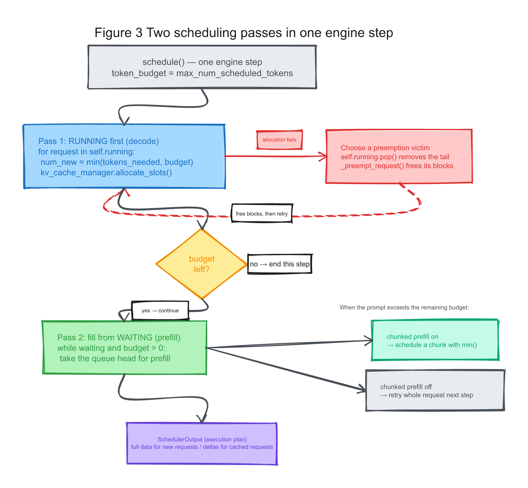
Figure: one
schedule()step. The scheduler considers running requests, admits waiting requests with any remaining budget, handles allocation failure through preemption, and packages the result asSchedulerOutput.
Pass 1: Why Running Requests Come First
The first substantive loop in schedule() traverses running
(scheduler.py:364):
# v1/core/sched/scheduler.py:364
# First, schedule the RUNNING requests.
req_index = 0
while req_index < len(self.running) and token_budget > 0:
    request = self.running[req_index]
    num_new_tokens = (request.num_tokens_with_spec
                      + request.num_output_placeholders
                      - request.num_computed_tokens)
    num_new_tokens = min(num_new_tokens, token_budget)
    ...
The source comments make the order explicit: running requests are considered before waiting requests. This ordering tends to protect inter-token latency for requests that are already generating, although the observed latency trade-off still depends on the configured scheduling policy and workload. It also lets requests that already hold KV blocks continue making progress toward completion and eventual reclamation. These are useful consequences of the order, not a claim that every running request always outranks every waiting request under all policies.
The waiting queue is an admission queue, not a tokenization cache. Requests in
it are waiting for scheduler resources; prompt preprocessing has already
happened before this point.
Pass 2: Chunked Prefill Is a Budget Clamp
After considering running requests, the scheduler uses any remaining budget to
admit work from waiting (scheduler.py:544). This is where the chunked-prefill
budget clamp appears.
A waiting request may have 5,000 prompt tokens while only 2,000 tokens remain in the current step’s budget. The relevant control flow is:
# Budget clamp inside the waiting loop
if (not self.scheduler_config.enable_chunked_prefill
        and num_new_tokens > token_budget):
    # If chunked_prefill is disabled, we can stop the scheduling here.
    break

num_new_tokens = min(num_new_tokens, token_budget)
assert num_new_tokens > 0
Two details matter here.
First, break does not drop the request. It exits the waiting-loop because the
remaining budget cannot admit another request in this step. The request stays
in waiting and is reconsidered the next time schedule() runs.
With chunked prefill enabled, min() admits the portion that fits and leaves
the rest for a later step. With it disabled, an over-budget request stays in
waiting and is retried as a whole. Neither path loses the request; removal
happens only after normal completion or an explicit abort.
A useful rule when reading schedulers is to ask where an item goes after a
break or continue. Here it remains in the same queue for a later step, just
as an OS process that misses one time slice remains runnable.
Second, chunked prefill reduces to a budget clamp:
num_new_tokens = min(num_new_tokens, token_budget). A long prompt contributes
only the tokens that fit in the current step; the remainder is scheduled later.
The full policy considers more state, but this clamp is what divides a long
prefill across scheduler steps.
(The running-request loop has the same clamp at scheduler.py:392. Because V1
does not maintain separate prefill and decode phases, the budget logic applies
uniformly to both.)
Preemption: Discard the KV State and Recompute
Another branch appears when a running request needs more KV blocks and
allocate_slots cannot satisfy the request. The allocation-retry loop beginning
at scheduler.py:443 can then preempt a victim:
# v1/core/sched/scheduler.py:443 (simplified)
while True:
    new_blocks = self.kv_cache_manager.allocate_slots(request, num_new_tokens, ...)
    if new_blocks is not None:
        break                              # Allocation succeeded; schedule normally
    # Allocation failed; choose a victim to preempt
    preempted_req = self.running.pop()      # Default policy: pop from the tail (LIFO)
    self._preempt_request(preempted_req, scheduled_timestamp)
    if preempted_req == request:
        break                              # No victim remains; defer this request
Under the default policy, self.running.pop() selects a victim from the tail
(LIFO). This usually victimizes a more recently admitted request with less
accumulated progress, reducing the work discarded, although queue position is
not a universal measure of recomputation cost. With PRIORITY
scheduling, victim selection also considers priority (scheduler.py:456).
_preempt_request (scheduler.py:929) defines what happens to the preempted
request’s KV-cache state:
# v1/core/sched/scheduler.py:929
def _preempt_request(self, request, timestamp):
    self.kv_cache_manager.free(request)          # ← release its KV blocks immediately
    self.encoder_cache_manager.free(request)
    request.status = RequestStatus.PREEMPTED
    request.num_computed_tokens = 0              # ← reset computed progress
    ...
    self.waiting.prepend_request(request)        # ← prepend it to the waiting queue
Two details matter here. First, num_computed_tokens = 0 records recomputation
semantics: the scheduler no longer treats the request’s previous progress as
resident KV state. When rescheduled, it must rebuild the required state, subject
to any cache reuse the current configuration can legitimately recover. This is
different from swapping the victim’s KV tensors to host memory and restoring
them later.
The trade-off is workload-dependent. Swapping consumes host-device bandwidth and host memory; recomputation consumes additional GPU work. vLLM V1 chooses the latter for this path, avoiding a KV transfer over PCIe at the cost of re-running model computation.
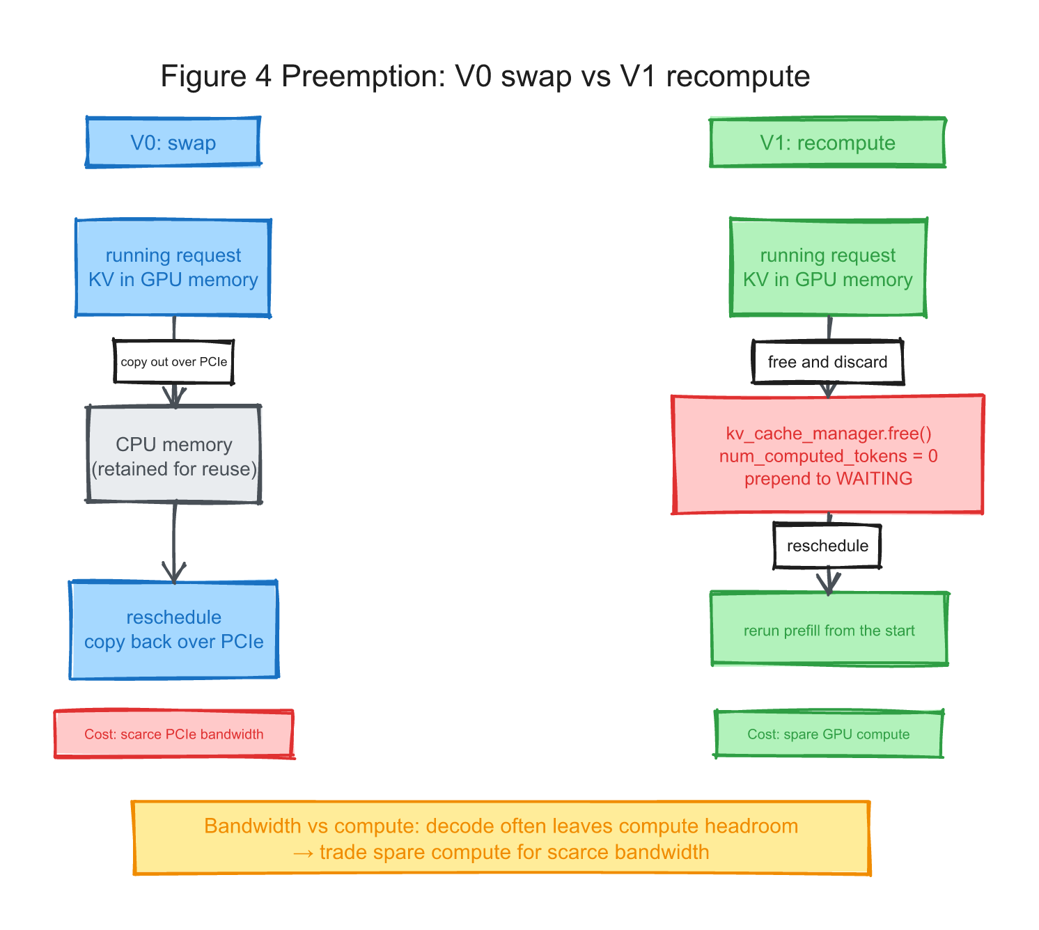
Figure: two preemption strategies. Swapping preserves KV state through a host-device transfer; recomputation releases the blocks and later rebuilds the required state.
The second detail is prepend_request, an anti-starvation measure. A preempted
request returns to the head of waiting rather than the tail. Appending it
behind every newly arrived request could cause repeated preemption and
indefinite delay; prepending gives the sacrificed request priority on the next
admission pass.
The Scheduler Produces SchedulerOutput
schedule() packages its decisions into SchedulerOutput (defined in
v1/core/sched/output.py:181) and hands that execution plan to the model
runner. The execution layer consumes the decision; it does not reschedule the
requests.
Many fields support optional features such as speculative decoding, multimodality, structured output, and connectors. Four core fields are enough to enter the execution layer:
# v1/core/sched/output.py:181 (selected core fields)
@dataclass
class SchedulerOutput:
    scheduled_new_reqs: list[NewRequestData]      # First scheduling: send complete request data
    scheduled_cached_reqs: CachedRequestData      # Previously scheduled: send only the delta
    num_scheduled_tokens: dict[str, int]          # req_id -> tokens processed in this step
    total_num_scheduled_tokens: int
    ...
    finished_req_ids: set[str]                     # Completed requests; tell the worker to reclaim state
    ...
    new_block_ids_to_zero: list[int] | None = None # Newly allocated blocks that the worker must zero
Their roles become clearer at the execution boundary.
scheduled_new_reqs carries the state needed when a request is first scheduled;
scheduled_cached_reqs carries updates for requests already known to the model
runner. This avoids rebuilding and transmitting the complete request state on
every step—a state-cache plus incremental-update pattern.
num_scheduled_tokens implements the unified progress model: it records how
many tokens each request will process in this step. The execution layer can use
those counts to pack prefill and decode work into one flat token batch.
finished_req_ids tells the worker which completed requests can release their
cached state, analogous to reclaiming OS resources after a process exits.
new_block_ids_to_zero identifies freshly allocated cache blocks that must be
cleared before the forward pass when KV-cache zeroing is enabled. Zeroing keeps
stale data or NaNs from an earlier owner from corrupting attention or
state-space-model computation. The field is conditional; not every
configuration needs this step.
Mapping the Scheduler to OS Concepts
Several scheduler concepts have useful operating-system analogies:
| Operating system concepts | vLLM Scheduler correspondence |
|---|---|
| Ready Queue | waiting |
| Run Queue | running |
| Physical page frame allocator | kv_cache_manager |
| Page fault/out of memory | allocate_slots returns None |
| Process swap | Preemption by releasing KV state and recomputing |
| time slice | token budget |
| Priority compensation after preemption | prepend_request returns the victim to the head of waiting |
| Output of scheduling decision | SchedulerOutput |
Continuous batching follows from rebuilding the execution batch at every
schedule() call. Completed requests leave, waiting requests enter, long
prompts may be split into chunks, and allocation pressure may trigger
preemption. The engine can therefore reuse newly available capacity without
waiting for an earlier fixed batch to finish in full.
Next, follow this SchedulerOutput plan into the execution layer and see how
variable-length requests become flat tensors for the model.
Part 3: Flattening Variable-Length Requests
The SchedulerOutput from the previous part reaches GPUModelRunner in the
worker. Suppose it assigns four tokens to request A and one token each to
requests B and C. How does the runner turn those unequal slices into tensors for
the GPU?
A conventional implementation might pad every request to the same length and
stack a [batch, seq_len] tensor. This path instead packs the scheduled tokens.
The path enters GPUModelRunner.execute_model
(v1/worker/gpu_model_runner.py:3913) and calls _prepare_inputs
(gpu_model_runner.py:1839). InputBatch
(v1/worker/gpu/input_batch.py:36) holds the prepared state:
# v1/worker/gpu/input_batch.py:36 (excerpt)
class InputBatch:
    req_ids: list[str]
    num_reqs: int

    # [num_reqs] tokens processed for each request in this step
    num_scheduled_tokens: np.ndarray
    # sum(num_scheduled_tokens): total tokens in this step
    num_tokens: int

    # [num_reqs + 1] request boundaries in the flattened sequence (prefix sum)
    query_start_loc: torch.Tensor
    # [num_reqs] current total length of each request, including history
    seq_lens: torch.Tensor

    # [num_tokens] ← one-dimensional, not [batch, seq_len]
    input_ids: torch.Tensor
    # [num_tokens]
    positions: torch.Tensor

    # [total_num_logits] positions that actually require logits
    logits_indices: torch.Tensor
The key shape is input_ids: [num_tokens]: the scheduled tokens form one
packed dimension rather than a padded batch matrix.
Flattening Requests into One Token Stream
V1 concatenates the tokens selected for the current step into one packed sequence, regardless of which request they belong to or whether they represent prefill or decode work.
In the example, A contributes a four-token prefill chunk, while B and C each contribute one decode token. If their current positions are 50 and 30, the packed tensors look like this:
input_ids   = [A0, A1, A2, A3, B0, C0]   # six values, one-dimensional
positions   = [ 0,  1,  2,  3, 50, 30]   # each token's position within its own request
A starts at position 0; B and C retain positions from their own sequences rather
than being renumbered within the packed batch. Here
num_scheduled_tokens = [4, 1, 1] and
query_start_loc = [0, 4, 5, 6]. The latter is a prefix sum that marks each
request’s range. Attention combines these boundaries with seq_lens to keep
requests separate.
This design has two advantages.
First, packing avoids computation on padding positions. Every scheduled position corresponds to actual request work, although kernels may still pad the packed token count internally for CUDA graphs or alignment.
Second, packing carries the scheduler’s unified token-count abstraction into
execution. The runner uses num_scheduled_tokens to place each request’s slice
in the flat sequence. Prefill and decode work can therefore coexist in one
step, while metadata preserves their separate boundaries.
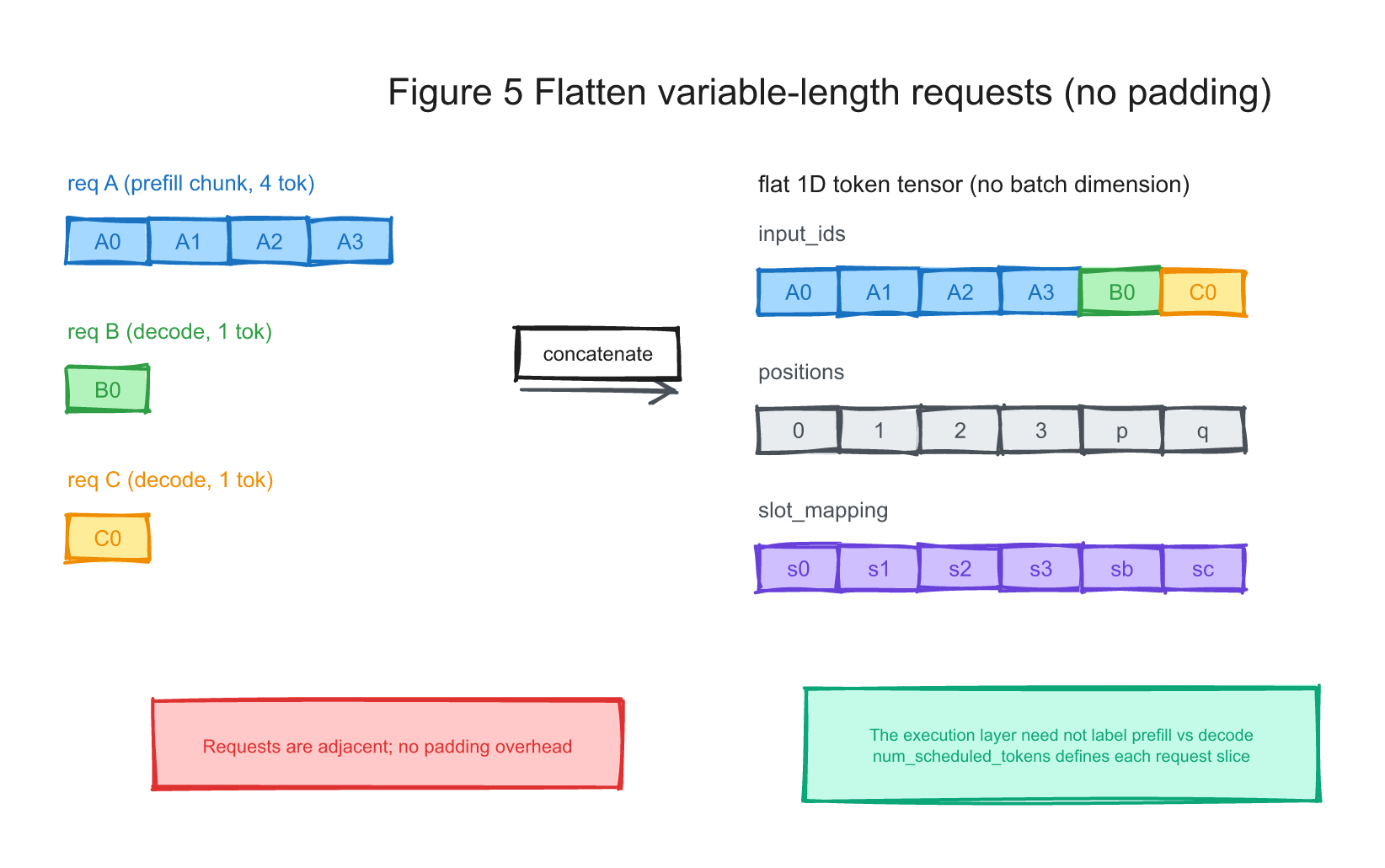
Figure: three variable-length requests—a prefill chunk and two decode requests—packed into one-dimensional
input_ids,positions, andslot_mappingarrays.
Two Values to Remember: slot_mapping and logits_indices
Two additional fields connect this packed representation to later stages.
slot_mapping is one-dimensional with shape [num_tokens], just like
input_ids. For every token in the current step, it records the destination
slot for the newly computed K and V tensors. Part 5 follows this value into the
KV-cache write kernel.
logits_indices has shape [total_num_logits], which can be much smaller than
num_tokens. To generate the next token, vLLM usually needs only the final
hidden state selected for each request. If a prefill chunk processes four
tokens, the first three positions do not need logits. logits_indices selects
only the positions that feed the sampler; Part 6 follows that path.
The model runner therefore produces a set of aligned flat views: input_ids
and positions feed the forward pass; query_start_loc and seq_lens delimit
requests for attention; slot_mapping selects KV-cache destinations; and
logits_indices selects the positions that require logits.
What This Part Established
- The execution layer packs scheduled request slices into one-dimensional
input_ids: [num_tokens]rather than a padded[batch, seq]matrix. query_start_locmarks request boundaries in the packed query, whileseq_lenssupplies each request’s visible KV length.num_scheduled_tokensconnects scheduler decisions to the packed execution batch, allowing prefill and decode work to coexist in one step.- Two values connect later stages:
slot_mappingselects KV destinations in Part 5, whilelogits_indicesselects the positions sampled in Part 6.
Next, the flat token sequence enters the model forward pass. The remaining question is how request boundaries and KV-block mappings reach attention operators buried inside many model layers.
Part 4: Passing Attention Metadata into Model Execution
The packed sequence now enters the model forward pass. Attention still needs step-specific metadata that does not appear in an ordinary model signature.
That metadata includes block_table, seq_lens, and query_start_loc. The
request set and lengths change each step, yet every attention layer needs access
to the corresponding state. How does it reach operators buried inside the
Transformer stack?
A direct design would pass the metadata through every layer:
forward(input_ids, attn_metadata), then layer(x, attn_metadata), then
attention(x, attn_metadata). In the OPT model definition, however, the
forward signature contains input_ids and positions but no
attn_metadata. The metadata enters through a different route.
Attention Metadata Lives in forward_context
The answer is in execute_model. The model’s forward is wrapped in a context manager and runs:
# Conceptual skeleton corresponding to execute_model in v1/worker
with set_forward_context(attn_metadata, self.vllm_config, ...):
    hidden_states = self.model(input_ids=input_ids, positions=positions)
set_forward_context (vllm/forward_context.py:250) installs
attn_metadata, slot_mapping, and related state in a scoped
forward_context while the model executes, then restores the previous context:
# vllm/forward_context.py:250 (structural excerpt)
def set_forward_context(attn_metadata, vllm_config, ..., slot_mapping=None, ...):
    forward_context = create_forward_context(
        attn_metadata, vllm_config, ..., slot_mapping, ...
    )
    try:
        with override_forward_context(forward_context):   # ← install the context globally
            yield                                          # ← model forward executes inside this scope
    finally:
        ...                                                # restore the previous context afterwards
The metadata therefore travels through scoped context rather than through every
model-layer signature. The ordinary forward path can keep tensor arguments such
as input_ids and positions while attention retrieves its runtime metadata
separately.
Deep inside the model, the attention layer retrieves that context. Consider
unified_attention_with_output
(model_executor/layers/attention/attention.py:734):
# model_executor/layers/attention/attention.py:734 (excerpt)
def unified_attention_with_output(query, key, value, output, layer_name, ...):
    layer_name = _resolve_layer_name(layer_name)
    # ↓ attn_metadata is retrieved rather than passed as an argument
    attn_metadata, self, kv_cache, _ = get_attention_context(layer_name)
    self.impl.forward(self, query, key, value, kv_cache, attn_metadata, output=output, ...)
The function receives layer_name, not attn_metadata directly.
get_attention_context(layer_name) resolves the layer and retrieves the
runtime state from forward_context (attention.py:648):
# model_executor/layers/attention/attention.py:648 (excerpt)
def get_attention_context(layer_name):
    forward_context = get_forward_context()          # ← retrieve the global context
    attn_metadata = forward_context.attn_metadata    # retrieve this layer's metadata by layer_name
    attn_layer = forward_context.no_compile_layers[layer_name]
    kv_cache = attn_layer.kv_cache
    slot_mapping = forward_context.slot_mapping.get(layer_name)
    return attn_metadata, attn_layer, kv_cache, slot_mapping
The resulting path is: execute_model installs the context, the model runs with
its normal tensor inputs, and each attention operator uses layer_name to
retrieve attn_metadata, kv_cache, and slot_mapping before dispatching to
self.impl.forward.
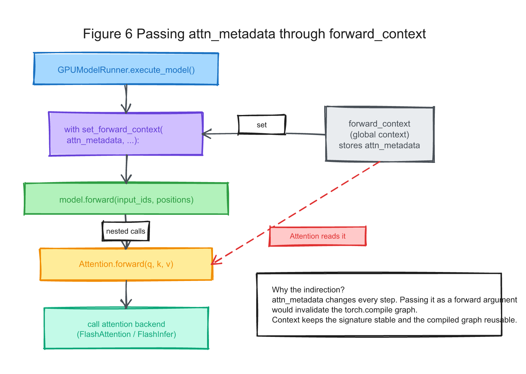
Figure:
execute_modelinstallsattn_metadatainforward_context; each attention layer retrieves its state bylayer_namebefore calling the backend.
Why This Indirection Helps torch.compile
Passing data through context is less explicit than ordinary arguments, but it
serves the compiled execution path. torch.compile benefits from stable graph
inputs and shapes; threading a changing Python metadata object through every
layer can introduce graph breaks, guards, or recompilation. Keeping that object
outside the model signature lets the compiled graph consume the tensor state it
needs through a controlled side channel. The exact compilation behavior still
depends on the selected backend and configuration, so this should be read as
the design goal rather than a guarantee that recompilation can never occur.
The Dummy Dependency That Preserves Ordering
unified_attention_with_output also accepts an apparently unused parameter,
kv_cache_dummy_dep. It is intentionally present and is not discarded in the
function body:
# attention.py:744
# kv_cache_dummy_dep is not used but accepting it creates a data dependency
# that ensures torch.compile preserves ordering between KV cache update and
# attention forward.
KV-cache update must precede the attention read, but mutation alone may not expose that ordering to the compiler. The dummy tensor makes the dependency explicit in the graph: the update produces a value consumed by attention, which prevents the two operations from being reordered across that edge.
What This Part Established
- Step-specific
attn_metadatastays out of the ordinary model-forward signature and is installed in a scopedforward_context. - Each attention layer retrieves its metadata, KV cache, and
slot_mappingthroughlayer_namebefore entering the backend. - This boundary is designed to make the model graph friendlier to
torch.compilewhile still exposing dynamic runtime state. - A dummy tensor dependency preserves the required update-before-read ordering for the KV cache.
The next part follows slot_mapping, block_table, and the KV cache into the
write and read paths.
Part 5: Writing and Reading the Paged KV Cache
PagedAttention is closely associated with vLLM, but the virtual-memory analogy alone does not identify the actual address structures. This part follows the write table and the read table in code.
The KV cache is a pool of fixed-size blocks rather than one contiguous region
per request. Each block stores K and V for block_size tokens (use
block_size=16 as a concrete example). A request’s logical token sequence may
span physically scattered blocks. This paging model removes the need to reserve
one large contiguous allocation for every request and substantially reduces
fragmentation from variable request lengths.
Here, block means a KV-cache allocation unit. Part 2 will also use CUDA thread blocks and matrix tiles; those are separate execution and computation concepts.
The two paths use different address structures: newly computed K/V is written by token, while attention reads a request’s history by logical cache block.
Write Path: One Token, One slot_mapping Entry
The previous part showed the attention layer retrieving slot_mapping from
forward_context. We can now follow it into the write kernel.
Each cache block contains block_size token slots. Flattening physical block
and in-block coordinates gives a cache-wide slot index:
physical_block_id × block_size + in_block_offset. slot_mapping, with shape
[num_tokens], gives that destination for every token processed in the step.
Under the FlashAttention and FlashInfer paths, KV writing finally falls to reshape_and_cache_flash (bound as ops.reshape_and_cache_flash in vllm/v1/attention/backends/fa_utils.py, defined in vllm/_custom_ops.py:2744):
# vllm/_custom_ops.py:2744
def reshape_and_cache_flash(
    key: torch.Tensor,          # K produced in this step
    value: torch.Tensor,        # V produced in this step
    key_cache: torch.Tensor,    # K block pool
    value_cache: torch.Tensor,  # V block pool
    slot_mapping: torch.Tensor, # ← destination slot for each token
    kv_cache_dtype: str,
    k_scale: torch.Tensor,
    v_scale: torch.Tensor,
) -> None:
Note: vLLM provides both
reshape_and_cacheandreshape_and_cache_flash, paired with different KV-cache layouts and read kernels. In V1, KV update is represented separately from the attention read; the dependency described in Part 4 preserves their required order under compilation.
For token i, the kernel reads the corresponding K and V vectors and writes
them to slot_mapping[i]. Decode commonly contributes one new position per
request; prefill contributes a chunk. The mapping is a per-token destination
table, not the data itself.
Read Path: One block_table per Request
Reading introduces logical-to-physical indirection. A query attends to visible
historical K/V positions that may be scattered across physical cache blocks;
block_table locates those blocks.
block_table is part of attn_metadata. For each request, entry j stores the
physical cache block backing logical block j. With block_size=16, logical
tokens 0–15 use the physical block named by block_table[0], tokens 16–31 use
block_table[1], and so on. This logical-to-physical array is the concrete
structure behind the page-table analogy.
On the GPU, the actual reading occurs in forward in the FlashAttention backend, which hands block_table directly to the flash kernel (vllm/v1/attention/backends/flash_attn.py:796):
# vllm/v1/attention/backends/flash_attn.py:758 (excerpt)
cu_seqlens_q = attn_metadata.query_start_loc
seqused_k    = attn_metadata.seq_lens
block_table  = attn_metadata.block_table
...
flash_attn_varlen_func(
    q=query[:num_actual_tokens],
    k=key_cache,
    v=value_cache,
    out=output[:num_actual_tokens],
    cu_seqlens_q=cu_seqlens_q,   # request boundaries in the flattened sequence (query_start_loc)
    seqused_k=seqused_k,         # history length of each request (seq_lens)
    block_table=block_table,     # ← page table: logical block → physical block
    ...
)
The GPU kernel follows block_table while loading the K/V history used by the
current query. The equivalent address translation is easier to see in the CPU
backend. The following excerpt is simplified from
csrc/cpu/cpu_attn_impl.hpp; the FlashAttention backend performs the same kind
of logical-to-physical lookup within its own tiled implementation:
// Simplified from the attention read loop in csrc/cpu/cpu_attn_impl.hpp
for (block_idx = start_block_idx; block_idx < end_block_idx; ++block_idx) {
    int physical_block_idx = block_table[block_idx];        // ← logical block number → physical block number
    kv_cache_t* k_cache_block_ptr =
        k_head_cache_ptr + physical_block_idx * kv_cache_num_blocks_stride;
    // Compute Q@K using K from this block ...
}
physical_block_idx = block_table[block_idx] is the essential page-table
lookup: traverse logical blocks in sequence, resolve each physical block, then
load K and V from that location.
Why the Write and Read Paths Use Different Addressing
In PagedAttention, two sets of addressing with different granularity are used for writing and reading.
Writes use slot_mapping at token granularity: each newly computed token has
one destination slot in the cache.
Reads use block_table at block granularity. Each request owns a sequence of
logical blocks whose entries identify the physical blocks containing its KV
history.
Keeping the two addressing schemes separate is what makes paging practical.
In the OS analogy, block_table is the page table, the block pool is physical
memory, and slot_mapping gives the physical destination for a write. It is
not a literal implementation of virtual memory, but the indirection is closely
related.
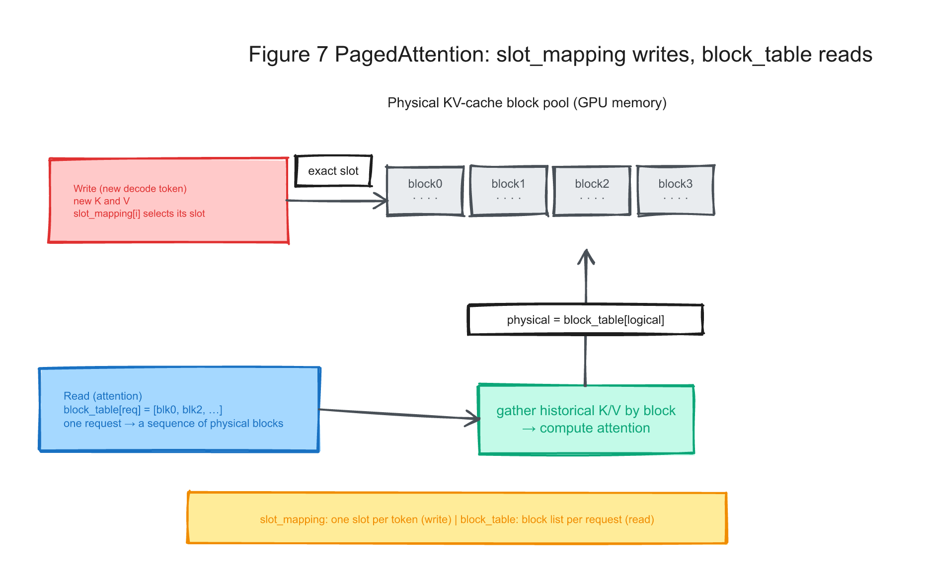
Figure:
slot_mappingsends each newly computed token to one physical cache slot, whileblock_tablemaps a request’s logical history to a sequence of physical blocks for reading.
What This Part Established
- The KV cache is a pool of fixed-size blocks. A request may occupy physically non-contiguous blocks. Paging substantially reduces external fragmentation, although the final partially filled block can still waste capacity.
- On write,
reshape_and_cache_flashusesslot_mapping: [num_tokens]to place each newly computed K/V pair in its destination slot. - Read:
block_tablestores the physical block numbers for each request. The GPU attention path uses it to resolvephysical = block_table[logical]while gathering the request’s KV history. - Writes use token-slot addresses; reads use logical-to-physical block mapping. The mechanism resembles virtual-memory paging, but it is a specialized KV allocator rather than a full virtual-memory implementation.
After attention consumes the updated cache, the model produces hidden states. The final part follows selected hidden states through logits and sampling, then shows how completed requests release their blocks.
Part 6: From Logits to Tokens and Block Reclamation
The model forward returns a packed set of hidden states. Only selected positions need logits for next-token sampling.
Compute Logits Only for the Required Positions
The logits_indices prepared in Part 3 now determines which hidden states are
projected into logits.
The model computes a hidden state for every scheduled token, but ordinary
next-token generation needs logits only at selected positions—typically the
last scheduled position for each request. For a four-token prefill chunk, the
first three hidden states therefore need not pass through lm_head for that
sampling step.
logits_indices selects those hidden states before the vocabulary projection.
Because lm_head projects into a vocabulary with tens or hundreds of thousands
of entries, avoiding unused positions saves substantial matrix-multiplication
work.
hidden_states[num_tokens]  --index_select(logits_indices)-->  keep only the required final position for each request
                           --lm_head-->  logits[num_reqs, vocab_size]
Sampling: From Logits to Token IDs
Sampler converts each vocab_size-dimensional logits vector into a token ID
according to temperature, top-p, top-k, or greedy selection.
The sampling results are packed into ModelRunnerOutput—whose central field is
sampled_token_ids—and sent back to EngineCore across the IPC boundary. This
completes the worker-side work for the scheduler step.
Return to the Scheduler: Append, Finish, and Recycle
When sampled_token_ids returns to EngineCore,
scheduler.update_from_output (v1/core/sched/scheduler.py:1283) performs the
third stage of EngineCore.step(): applying model output to request state.
First, take out the new token:
# scheduler.py:1363 (excerpt)
req_index = model_runner_output.req_id_to_index[req_id]
generated_token_ids = sampled_token_ids[req_index] if sampled_token_ids else []
Second, _update_request_with_output appends the new token and evaluates stop
conditions such as EOS, max_tokens, and configured stop strings:
# scheduler.py:1407 (excerpt)
if new_token_ids:
    new_token_ids, stopped = self._update_request_with_output(request, new_token_ids)
Third, when a request stops, its KV blocks are returned to the pool:
# scheduler.py:1474 (excerpt)
if stopped:
    finish_reason = request.get_finished_reason()
    finished = self._handle_stopped_request(request)
    if finished:
        kv_transfer_params = self._free_request(request)   # ← release its KV blocks
    ...
    stopped_running_reqs.add(request)
After the cycle ends, remove these stopped requests from the running queue:
# scheduler.py:1528 (excerpt)
if stopped_running_reqs:
    self.running = remove_all(self.running, stopped_running_reqs)
This closes the continuous-batching loop. When a request finishes,
_free_request returns its blocks to the pool and removes one entry from
running. On the next step, schedule() can spend those blocks on requests in
waiting. Resource reclamation is therefore part of admission control, not an
unrelated cleanup detail.
An unfinished request remains eligible in running; a later scheduling step can
advance it again.
Finally, EngineCore packages the results as EngineCoreOutputs and sends them
to the main process over IPC. LLMEngine.step() consumes them through
get_output(), detokenizes token IDs, assembles RequestOutput, and returns it
to the caller. That completes the path from an API request to generated text.
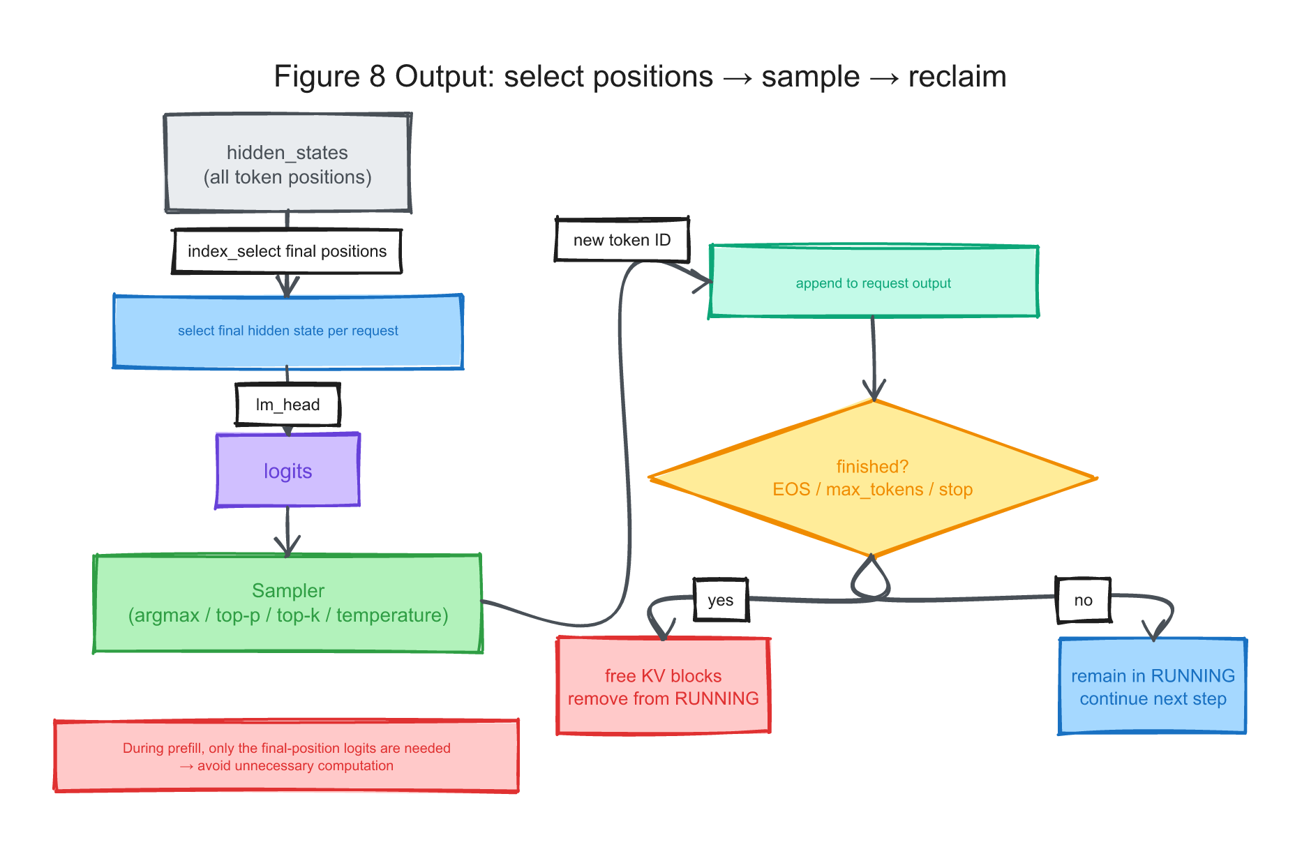
Figure:
logits_indicesselects the required hidden states,lm_headproduces logits, and sampling yields new token IDs. Finished requests release their KV blocks; unfinished requests remain active.
What This Part Established
logits_indicesselects the positions that require vocabulary projection, avoidinglm_headwork for unused intermediate positions.Samplerproduces token IDs according to each request’s sampling parameters and returns them inModelRunnerOutput.update_from_outputappends new tokens, evaluates stopping conditions, and calls_free_requestfor completed requests.- Reclaimed KV capacity becomes available to later scheduler steps.
What to Carry Forward
The six parts reduce vLLM’s request path to a scheduler, a paged memory manager, and a GPU execution pipeline. Four design choices are especially reusable:
First, the scheduler expresses both prefill and decode as per-request token progress. The execution layer then packs those scheduled tokens into one dimension. Chunked prefill and continuous batching build on the same contract instead of requiring separate batch formats.
Second, V1 preempts by recomputing rather than swapping. Under KV-cache
pressure, it frees the victim’s blocks, resets num_computed_tokens, and
requeues the request for prefill instead of moving KV state to CPU memory and
back over PCIe. This trades additional computation for less host-device data
movement.
Third, forward_context keeps step-specific attn_metadata out of the forward
signature so torch.compile can reuse a stable graph. A dummy tensor dependency
then constrains operator ordering. The indirection is less obvious to read, but
it serves compilation and execution correctness.
Fourth, writes are addressed per token while reads are resolved per block.
slot_mapping selects each token’s write slot; block_table maps a request’s
logical KV blocks to physical blocks. At its core, the page-table lookup is
physical = block_table[logical].
The same discipline appears throughout the path: identify whether the scarce
resource is compute, bandwidth, KV capacity, TTFT, or inter-token latency, then
make the trade-off explicit. vLLM’s throughput does not come from one isolated
trick. It comes from small mechanisms that compose: a budget clamp expressed by
min, one level of block_table indirection, and a deliberate
num_computed_tokens = 0 on preemption.
What this article doesn’t cover
To keep the path traceable, this article stops at the Python/CUDA boundary. It does not cover:
- CUDA and Triton kernel internals. We stop at the attention-backend call rather than tracing tiling and online softmax.
- Block-allocation details inside
kv_cache_manager, including reference counting and prefix-cache hash reuse. The article treats it only as a block allocator. - Multi-GPU parallelism: communication and partitioning under tensor (TP), pipeline (PP), and data parallelism (DP).
- Advanced features such as speculative decoding, multimodality, and structured
output. Their state appears in
SchedulerOutput, but they are outside this request path.
This walkthrough targets the vLLM 0.22.0 V1 architecture. Source locations are included so readers can compare the excerpts with their installed version. The editable Excalidraw sources for Figures 2–8 are published with this site.