Part 3 · vLLM internals
Building a Verifiable FlashAttention Forward from PyTorch to Triton
This English edition is adapted from the published Chinese article on Zhihu. It preserves the source-code references, experimental boundaries, and reproducible artifacts while adapting the structure for an international engineering audience.
Part 2 identified the stable data flow behind FlashAttention: keep a Q tile on-chip, stream K/V tiles through it, update online softmax, and write only the final output. This article turns that data flow into executable code. It begins with explicit PyTorch attention, validates the tiled recurrence in PyTorch, then moves QK, softmax, and P·V into one Triton forward kernel.
The intended reader knows the attention equation and basic GPU concepts such as tiles, global memory, and kernel launches. No prior Triton implementation experience is required; the article introduces the small set of Triton concepts needed to follow the kernel, but it is not a general Triton tutorial.
Scope. This is a compact inference-forward implementation for
contiguous [B, H, N, D] self-attention. It supports FP16/BF16,
causal/non-causal attention, and head dimensions 64 and 128. It deliberately
omits backward, dropout, GQA, variable-length inputs, paged KV, split-KV, and
architecture-specific pipelines.
Measured environment. NVIDIA GeForce RTX 4090 24 GB, driver 580.105.08, Python 3.12.3, PyTorch 2.5.1+cu124, and Triton 3.1.0. All correctness and performance results come from this environment. Raw logs and CSV files are in the companion repository.
From a Data-Flow Sketch to an Executable Kernel
The previous article reduced FlashAttention to four data-flow steps:
Keep one Q tile on-chip
    ↓
Stream K/V tiles through a loop
    ↓
Update online softmax and the P·V accumulator
    ↓
Write only the final output to global memory
The data flow is compact, but two questions must be answered before it becomes a trustworthy kernel:
- Algorithm: how can softmax contributions from multiple K/V tiles be combined exactly without storing the full score matrix?
- Engineering: how should that tiled loop be fused into one kernel, and how do we verify its boundaries, numerical behavior, and performance?
The implementation proceeds in five stages:
- Explicit PyTorch: establish a numerical reference and expose the full
N×Nintermediate matrix. - Tiled PyTorch: validate online softmax without claiming a speedup.
- Fused Triton: move the K/V loop into one kernel and eliminate repeated launches and intermediate write-backs.
- Correctness: cover dtype, masking, boundary shapes, and stability.
- Measurement: compare latency and peak memory with both eager attention and production PyTorch SDPA.
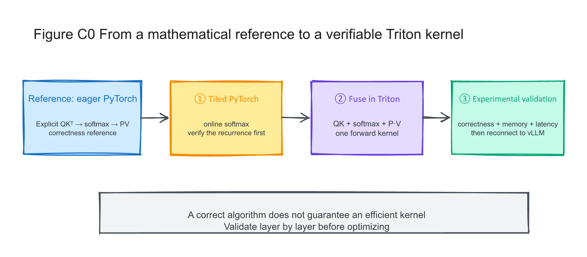
Figure C0: eager PyTorch provides the numerical reference, tiled PyTorch validates the recurrence, and Triton fuses that recurrence into one kernel. Correctness, memory, and latency are measured before reconnecting the result to vLLM’s production path.
The complete runnable implementation is in
flash_attention_lab.py.
The article includes only the code that determines data flow; argument checks
and benchmark scaffolding remain in the repository.
Part 1: Explicit PyTorch Attention and Its Intermediate State
The formula for Scaled Dot-Product Attention has not changed:
S = QKᵀ / sqrt(D)  # similarity between each query and all keys
P = softmax(S)     # normalize each row across key positions
O = PV             # weighted sum of value vectors
Here D is one head’s dimension and N is the sequence length. For each
(batch, head), Q/K/V have shape [N, D], S/P have shape [N, N], and O has
shape [N, D].
First write it explicitly in PyTorch:
def attention_torch(q, k, v, *, causal):
    d = q.shape[-1]  # Per-head dimension D

    # [B,H,N,D] @ [B,H,D,N] -> [B,H,N,N]
    # Use FP32 scores as the numerical reference.
    scores = torch.matmul(q.float(), k.float().transpose(-1, -2))
    scores *= 1.0 / math.sqrt(d)  # 1/sqrt(D) in scaled dot-product

    if causal:
        n = q.shape[-2]
        # triu(1) marks key positions strictly later than each query.
        future = torch.ones((n, n), dtype=torch.bool, device=q.device).triu(1)
        # Softmax assigns zero probability to positions masked with -inf.
        scores.masked_fill_(future, float("-inf"))

    probs = torch.softmax(scores, dim=-1)  # Normalize across key positions
    # [B,H,N,N] @ [B,H,N,D] -> [B,H,N,D]
    return torch.matmul(probs, v.float()).to(q.dtype)
The reference promotes Q and K to FP32 before computing scores. This improves
its usefulness as a numerical reference but also enlarges the intermediate
matrices. For input [B, H, N, D]:
Q / K / V: [B, H, N, D]
scores  : [B, H, N, N]
probs   : [B, H, N, N]
output  : [B, H, N, D]
When B=1, H=16, the theoretical size of just one FP32 scores matrix is:
| N | Single [B,H,N,N] FP32 matrix |
|---|---|
| 512 | 16 MiB |
| 1024 | 64 MiB |
| 2048 | 256 MiB |
| 4096 | 1024 MiB |
| 8192 | 4096 MiB |
If both scores and probs are live, their combined storage is twice the value
in the table. Exact FlashAttention still computes the QK terms; its advantage is
that these two full matrices need not be written to and read from global memory.
It is still too broad to label every attention workload “memory-bound.” The
actual bottleneck depends on sequence length, head dimension, GPU, dtype, and
whether the workload is prefill or decode. FlashAttention keeps exact
attention’s O(N²D) arithmetic complexity; it reduces HBM traffic and avoids
quadratic-size score/probability storage.
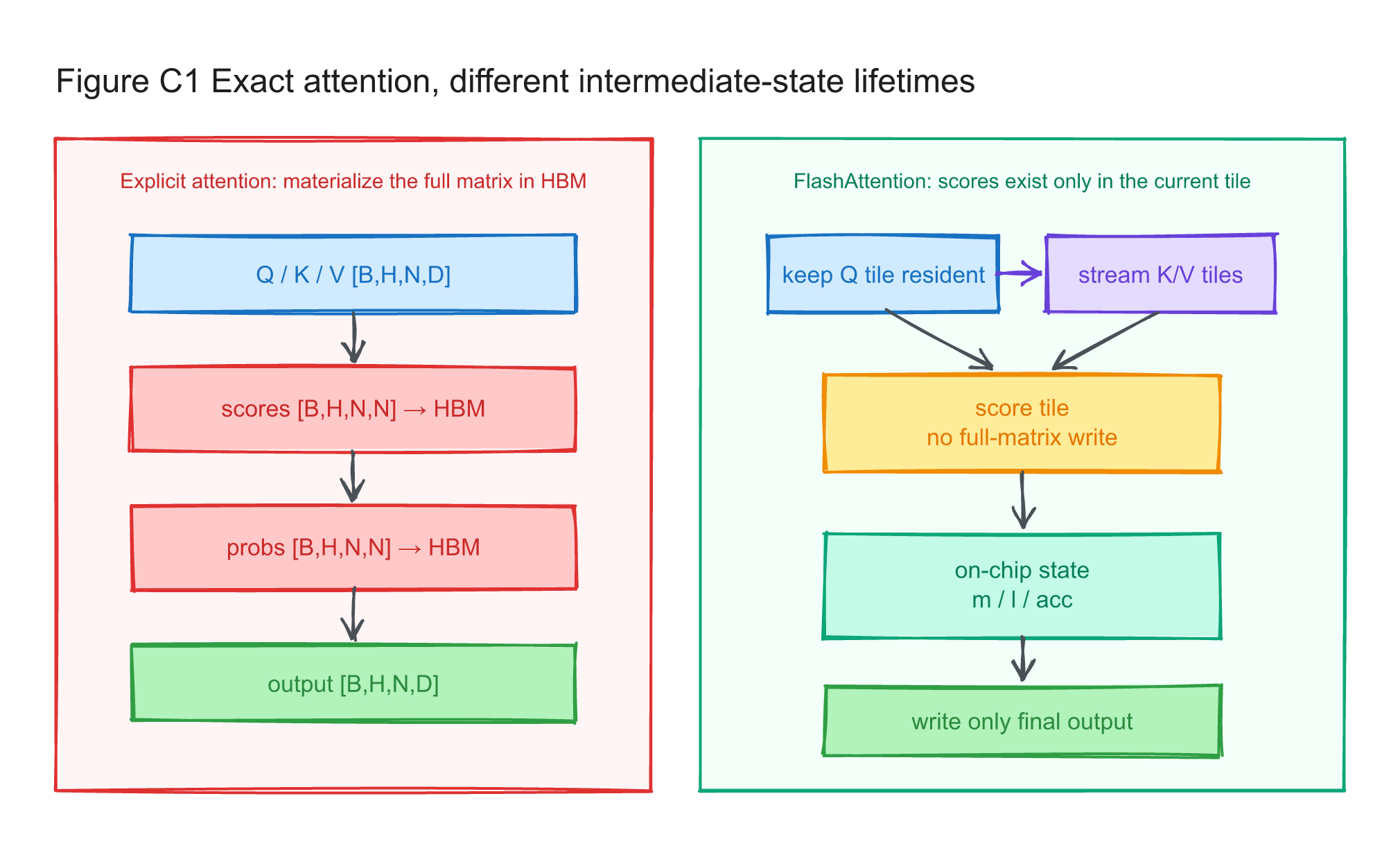
Figure C1: explicit attention materializes full score and probability matrices in HBM. The tiled path retains only the current score tile and the per-row
m/l/accrecurrence state before writing the final output.
Why not use PyTorch SDPA as the formula reference?
torch.nn.functional.scaled_dot_product_attention is a dispatcher. PyTorch may
select a fused FlashAttention, memory-efficient, or math backend according to
device, dtype, shape, and mask. It is useful as a production baseline, but it
does not expose the explicit intermediate state needed to validate this
derivation.
The experiments therefore use two PyTorch comparisons:
- Explicit
QKᵀ -> softmax -> PVabove: correctness reference and eager baseline; F.scaled_dot_product_attention: production framework baseline, used to measure the remaining gap to PyTorch’s selected implementation.
The target is now clear: QK work remains, but full score and probability matrices should not live in HBM. Before writing Triton, solve the mathematical problem: if only one score tile is visible at a time, how can we recover exactly the same result as a full-row softmax?
Part 2: Tiled PyTorch and Online Softmax
Reducing Full Softmax to Three Running States
For a row of logits x, stable softmax is usually written as:
m = max_j(x_j)                 # largest logit in the row
l = Σ_j exp(x_j - m)           # softmax normalization denominator
softmax(x_i) = exp(x_i - m) / l
The subscript j spans all key positions in the row. Subtracting m leaves the
normalized result unchanged because numerator and denominator receive the same
factor. It also makes the largest exponential exp(0)=1, preventing overflow
from a large positive logit.
A conventional stable softmax first finds the maximum over the entire row and then sums the shifted exponentials, which appears to require retaining all scores. Tiling removes that global view: while processing the first K tile, a larger value may still appear later. Online softmax must rescale the accumulated state whenever that running maximum changes.
The full score row is not required. After processing part of K/V, retain three pieces of running state:
m_old: the largest logit seen so far; a scalar for each Q row
l_old: sum of shifted exponentials under m_old; one scalar per Q row
acc_old: Σ exp(score - m_old) · V; one D-dimensional vector per Q row
After the new scores tile arrives:
m_tile = row_max(scores_tile) # The maximum value of each row of the current tile
m_new = max(m_old, m_tile) # The common maximum value of historical and current tiles

alpha = exp(m_old - m_new) # Scale the historical state to the new baseline
p = exp(scores_tile - m_new) # The weight of the current tile that has not yet been normalized

l_new = alpha · l_old + row_sum(p)     # combine old and new normalization sums
acc_new = alpha · acc_old + p · V_tile # combine old and new weighted values
The last piece is processed:
output = acc / l # numerator and denominator use the same shifted basis
Because m_new >= m_old, alpha lies in (0, 1]. If the running maximum
increases, multiplying the old l and acc by
exp(m_old - m_new) expresses them under the new shifted baseline. p contains
unnormalized weights for the current tile, not final probabilities. Since l
and acc use the same baseline, the final division cancels the common scale.
Only m, l, and acc must survive between tiles.
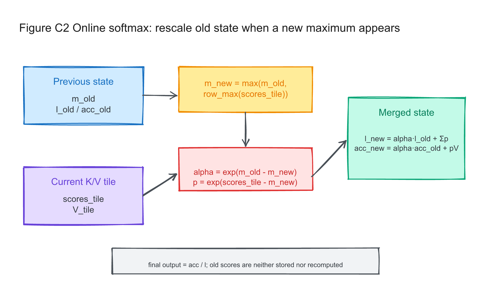
Figure C2: when a new KV tile raises the running maximum,
alpharescalesl_oldandacc_oldto the new baseline before the current tile’spandp·Vcontributions are added.
Verify the Recurrence in PyTorch First
Deriving the recurrence is not enough; masks, broadcast dimensions, and tail
tiles are easy to get wrong. The reference implementation selects a Q tile in
the outer loop and scans K/V tiles in the inner loop. Its
running_max, running_sum, and acc variables correspond to m, l, and
the output accumulator above:
for m_start in range(0, n, block_m):
    m_end = min(m_start + block_m, n)  # The last Q tile may not be block_m rows long
    rows = m_end - m_start
    q_tile = q[:, :, m_start:m_end, :].float()

    # Each Q row has its own m, l, and D-dimensional accumulators.
    running_max = full([B, H, rows], -inf)  # Corresponds to m in the formula
    running_sum = zeros([B, H, rows])       # Corresponds to l in the formula
    acc = zeros([B, H, rows, D])            # unnormalized weighted value

    for n_start in range(0, n, block_n):
        n_end = min(n_start + block_n, n)  # The last KV tile may also be incomplete
        k_tile = k[:, :, n_start:n_end, :].float()
        v_tile = v[:, :, n_start:n_end, :].float()
        # [B,H,rows,D] @ [B,H,D,cols] -> [B,H,rows,cols]
        scores = q_tile @ k_tile.transpose(-1, -2) * scale

        if causal:
            # A query may attend only to keys at the same or earlier positions.
            scores.masked_fill_(kv_pos > q_pos, -inf)

        tile_max = scores.amax(dim=-1)                  # m_tile
        new_max = maximum(running_max, tile_max)        # m_new
        alpha = exp(running_max - new_max)              # Recalibrate old state
        p = exp(scores - new_max.unsqueeze(-1))         # Unnormalized weights for this tile

        # alpha.unsqueeze(-1) expands [B,H,rows] to [B,H,rows,1],
        # Apply the same row-wise coefficient to all D accumulator elements.
        acc = acc * alpha.unsqueeze(-1) + p @ v_tile
        running_sum = running_sum * alpha + p.sum(dim=-1)
        running_max = new_max

    # Only perform normalization once after scanning all KV tiles.
    output[:, :, m_start:m_end, :] = acc / running_sum.unsqueeze(-1)
This version no longer materializes a full [N, N] score matrix, but it is not
expected to be fast. Each PyTorch operator may launch one or more GPU kernels,
and the nested Python loops multiply launch overhead and intermediate tile
traffic.
Its purpose is to separate failure domains:
- If it disagrees with eager attention, inspect the recurrence and mask.
- If tiled PyTorch agrees but Triton does not, inspect program mapping, pointer arithmetic, bounds, and precision.
- If both are correct but Triton is slow, investigate tiling, warps, occupancy, and memory traffic.
The next step keeps the recurrence unchanged and moves the inner K/V loop across the execution boundary: from a sequence of PyTorch operations into one Triton kernel.
Part 3: Move the Same Recurrence into One Triton Kernel
The One Triton Concept You Need: A Program Processes a Tile
This section introduces only the Triton concepts needed for the kernel. CUDA code is often read by asking which values individual threads handle; Triton is usually read by asking which tile one program instance handles.
The host launches a grid of program instances
    ↓
Each program instance handles one or more data tiles
    ↓
The program expresses vector and matrix operations over its tile
    ↓
The compiler maps those operations to warps, memory accesses, and instructions
Only a small set of Triton primitives appears repeatedly:
| Symbol | Meaning here | Closest CUDA analogy |
|---|---|---|
@triton.jit |
Compile a Python-defined function as a GPU kernel | Kernel compilation entry |
tl.program_id(axis) |
Index of the current program in one launch-grid dimension | Closer to CUDA’s blockIdx than threadIdx |
tl.arange(0, BLOCK) |
Generate logical coordinates within a tile | Vector of indices, not a new set of threads |
Pointer expression + tl.load/tl.store |
Form addresses from base pointers, strides, and coordinates | Load or store a tile with masks |
mask=... |
Disable out-of-bounds or semantically invalid elements | Apply a predicate across coordinates |
tl.dot(a, b) |
Matrix product over two blocks | Tile-level GEMM; the compiler selects the hardware path |
tl.constexpr |
Parameters known at launch time for compile-time specialization | Generate specialized kernels for different head sizes, tile sizes, or causal branches |
When reading tl.arange, identify the coordinates it creates for the current
program. Read tl.dot as a tile matrix multiplication. The launch mapping here
is:
program_id(0) -> which Q tile
program_id(1) -> flattened (batch, head) index
The grid is:
# The first dimension covers all Q tiles, and the second dimension expands all (batch, head).
grid = (triton.cdiv(N, BLOCK_M), B * H)
A program is responsible for:
fixed batch_id
fixed head_id
one Q-row tile: [BLOCK_M, D]
loop over K/V tiles: [BLOCK_N, D]
write one output tile: [BLOCK_M, D]
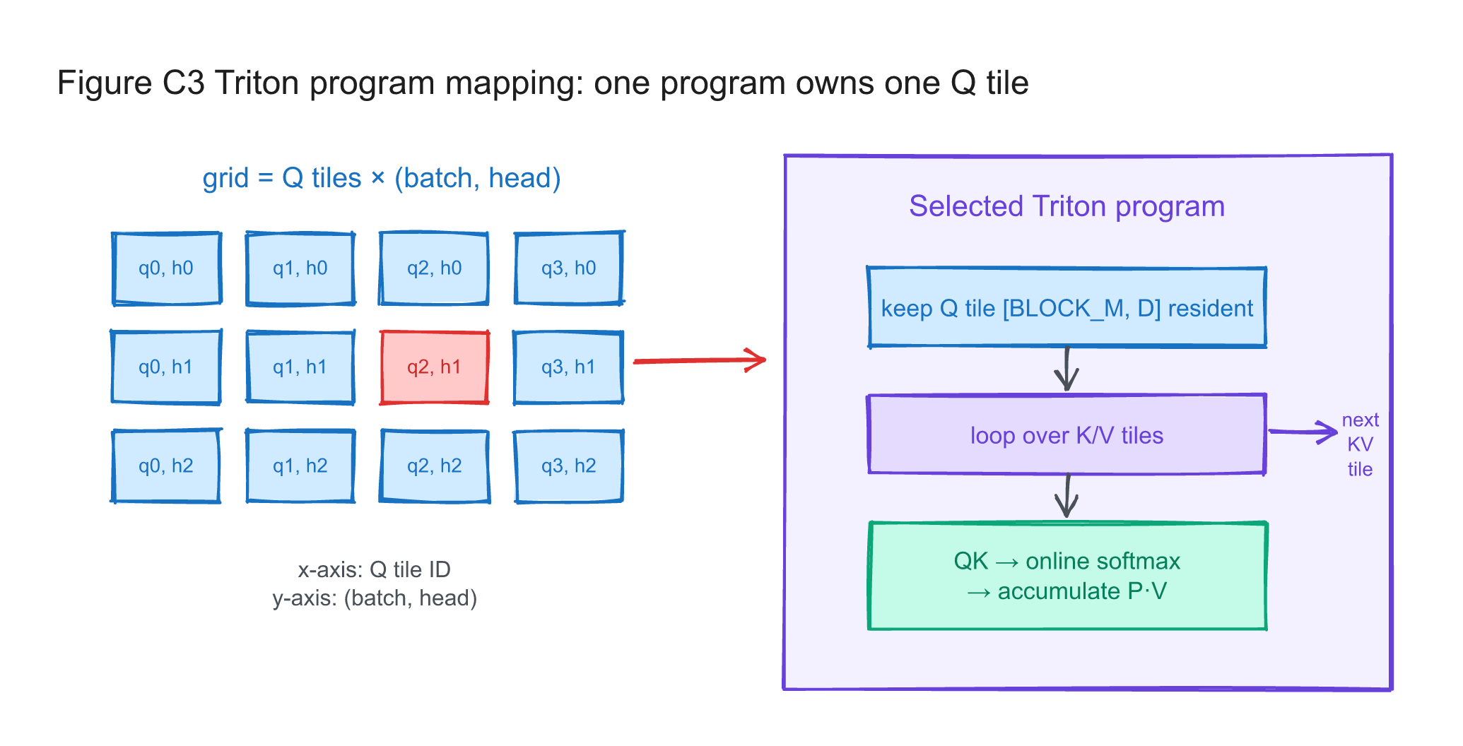
Figure C3: the Triton grid spans
(batch, head)pairs and Q tiles. Each program owns one Q tile and scans K/V tiles internally; programs write disjoint output rows and do not synchronize with one another.
The kernel now follows the data flow from Part 2: load one Q tile, initialize
m/l/acc, scan K/V tiles, then write the normalized output.
Step 1: Select and Load a Q Tile
The program first recovers the batch and head indices, then constructs row and feature coordinates:
pid_m = tl.program_id(0)   # Q-tile index
pid_bh = tl.program_id(1)  # Flattened (batch, head) index
batch_id = pid_bh // n_heads
head_id = pid_bh % n_heads

offs_m = pid_m * block_m + tl.arange(0, block_m)  # [BLOCK_M] query positions
offs_d = tl.arange(0, head_dim)                    # [D] feature positions
The tensor strides form the address matrix:
q = tl.load(
    q_base
    # Broadcast [BLOCK_M,1] and [1,D] into a [BLOCK_M,D] address grid.
    + offs_m[:, None] * stride_qn
    + offs_d[None, :] * stride_qd,
    mask=offs_m[:, None] < n_ctx,  # Ignore tail rows outside the sequence.
    other=0.0,                     # Masked elements return 0 without a memory read.
)
The mask handles a final Q tile with fewer than BLOCK_M valid rows. The
program keeps q live while scanning all visible K/V tiles.
Step 2: Initialize the Cross-Tile State
The state matches the tiled PyTorch version:
row_is_valid = offs_m < n_ctx                              # [BLOCK_M]
m_i = tl.where(row_is_valid, -float("inf"), 0.0)           # running max per row
l_i = tl.zeros((block_m,), dtype=tl.float32)               # normalization sum per row
acc = tl.zeros((block_m, head_dim), dtype=tl.float32)      # [BLOCK_M,D]
m_i and l_i are one scalar per Q row, and acc is one D-dimensional vector per Q row. They are retained as on-chip state within the loop and are not written as global intermediate tensors.
Invalid rows in the final Q tile initialize m_i to zero rather than negative
infinity. Otherwise their first update would evaluate
-inf - (-inf) inside alpha and produce NaN even though the final store is
masked. A valid causal row always has at least one visible key in its first K/V
tile—at minimum its own position—so its row maximum is finite.
Step 3: Stream K/V Tiles through the Loop
Causal attention never needs keys beyond the right edge of the current Q tile:
end_n = n_ctx  # non-causal requires scanning the complete KV sequence
if is_causal:
    # The rightmost query in this tile cannot attend beyond this boundary.
    end_n = tl.minimum(n_ctx, (pid_m + 1) * block_m)

for start_n in tl.range(0, end_n, block_n):
    current_n = start_n + tl.arange(0, block_n)  # Absolute K/V positions
    ...
Each iteration loads [BLOCK_N, D] K and V tiles. The
current_n < n_ctx mask handles the tail before computing a
[BLOCK_M, BLOCK_N] score tile:
# [BLOCK_M,D] @ [D,BLOCK_N] -> [BLOCK_M,BLOCK_N]
qk = tl.dot(q, tl.trans(k)) * scale_log2

# Two 1D masks are broadcast into the same 2D shape as qk.
valid = row_is_valid[:, None] & kv_is_valid[None, :]
if is_causal:
    # Mask keys whose positions are later than the query position.
    valid &= current_n[None, :] <= offs_m[:, None]
qk = tl.where(valid, qk, -float("inf"))  # exp2(-inf) = 0
There are two types of masks:
- Boundary mask: handles sequence lengths that are not tile multiples.
- Causal mask: permits only
kv_position <= query_position.
The boundary mask usually affects only the final tile. The causal mask forms a
triangle within diagonal tiles, while end_n skips K/V tiles entirely to the
right of the current Q tile.
Step 4: Update Online Softmax in the Loop
To use exp2, fold log2(e) into the QK scale:
exp(x) = e^x = 2^(x · log2(e))
This changes only the exponential base. Folding log2(e) into the QK scale
lets the kernel use exp2 while computing the same softmax weights.
This makes m_i a running maximum of logits already scaled into base-2
exponent units. l_i is still an ordinary, dimensionless sum of shifted
weights; it is not a logarithm. A future split-KV implementation that exports
log-sum-exp state must keep the logarithm base and scale consistent across its
partial and combine kernels.
The wrapper passes:
scale_log2 = (1.0 / sqrt(D)) * log2(e) # softmax scale × base conversion
The recurrence in the kernel corresponds directly to the previous part:
tile_max = tl.max(qk, axis=1)              # Per-row maximum in this tile
m_new = tl.maximum(m_i, tile_max)          # Updated running maximum
alpha = tl.math.exp2(m_i - m_new)          # [BLOCK_M], rescale prior state
p = tl.math.exp2(qk - m_new[:, None])      # [BLOCK_M,BLOCK_N], not yet normalized

# Convert p to V's dtype for tl.dot; accumulate the output in FP32.
acc = acc * alpha[:, None] + tl.dot(p.to(v.dtype), v)
l_i = l_i * alpha + tl.sum(p, axis=1)      # Update the normalization sum
m_i = m_new
Normalize and write back only after the loop ends:
# Broadcast the row-wise denominator across D output dimensions.
output = acc / l_i[:, None]
# Store only valid Q rows; out-of-bounds tail rows perform no write.
tl.store(output_ptrs, output, mask=row_is_valid[:, None])
Looking at the three implementations side by side, the math hasn’t changed:
| Version | Score-tile lifetime | Location of the K/V loop | Kernel launches |
|---|---|---|---|
| Eager PyTorch | Full [N, N] score matrix is materialized in HBM |
No explicit loop | A few large operators |
| Tiled PyTorch | Only the current tile is explicit, but operator boundaries may spill state to HBM | Python | Multiple launches per tile |
| Triton | Current tile and recurrence state remain inside one program instance | Kernel | One fused launch for the forward pass |
Online softmax makes exact attention tileable; fusion determines whether the intermediate tile state remains on chip or repeatedly crosses a global-memory boundary. The algorithm and the execution boundary solve different halves of the problem.
Part 4: Establish Correctness Before Measuring Speed
Once the recurrence moves into a kernel, program mapping, tail masks, causal
boundaries, and low-precision arithmetic become the main sources of error. The
test matrix therefore includes lengths around tile boundaries rather than only
an aligned N=1024 case.
Why Test Sequence Lengths 127, 128, and 129?
For tile sizes such as 64 or 128:
- 128 lands exactly on a tile boundary.
- 127 exercises a one-element-short tail.
- 129 launches an additional tile with only one valid row or column.
Testing only aligned sizes can leave broken boundary masks undetected.
The script covers:
| dimensions | case |
|---|---|
| sequence length | 127, 128, 129, 511, 512, 1024 |
| head dimension | 64, 128 |
| dtype | FP16, BF16 (when supported by hardware) |
| mask | causal, non-causal |
| batch/head | 2×8 for small sequences and 1×4 for large sequences |
| stability | N=513, with Q/K magnified 4× |
Execution:
python flash_attention_lab.py check
The reference uses explicit FP32 PyTorch attention. Tolerances differ by dtype:
BF16 needs a wider tolerance because it has fewer mantissa bits than FP16. Each
case reports maximum and mean absolute error, then applies
torch.testing.assert_close.
The amplified Q/K case stresses softmax stability. A direct exp(scores) is
more likely to overflow, while subtracting the running maximum should keep the
result finite. The test therefore checks both closeness and finiteness:
# Reject NaN and either sign of infinity.
assert torch.isfinite(actual).all()
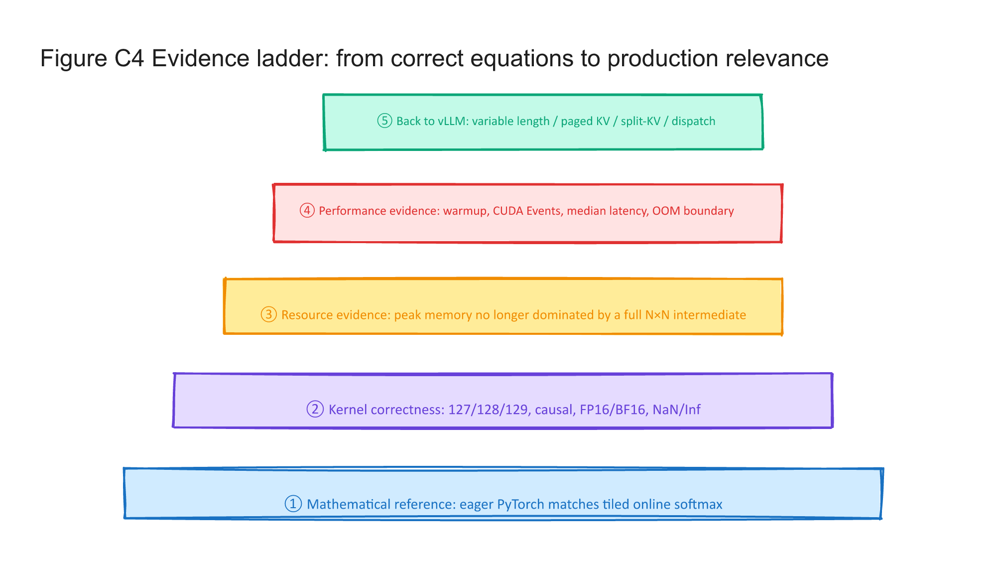
Figure C4: verification proceeds from recurrence and boundary correctness to numerical checks, memory and latency measurement, and comparison with the production vLLM path.
A total of 71 cases passed the supplemental test suite:
- 8 tiled-PyTorch comparisons with the eager reference;
- 48 Triton dtype/mask/shape combinations;
- 1 stability case at
N=513with Q/K amplified 4×; - 6 long-sequence cases at
N=2048/4096/8192; - 8 checks of FP16 eager and Flash-only SDPA against the FP32 reference.
Across these runs, maximum absolute error stayed at or below 0.001953 for
FP16 and 0.015625 for BF16. Every case met its dtype-specific
assert_close tolerance, and the stability case contained no NaN or infinity.
assert_close applies both absolute and relative tolerances. A standalone
maximum relative-error statistic is not reported because outputs near zero can
make that ratio arbitrarily large; a future report should pair relative error
with output-magnitude bins if it needs that diagnostic.
The complete output is in
results/supplemental/correctness.log.
Agreement in tiled PyTorch validates the recurrence; agreement in Triton then
checks program mapping, masks, and numerical behavior together.
Part 5: Benchmarking Fusion and Memory Traffic
After correctness is established, five paths separate three questions that the original four-way comparison mixed together: numerical-reference behavior, same-precision eager execution, and the gap to a named production backend.
eager_fp32_ref   explicit FP32 score/probability reference
eager_fp16       unfused eager attention with FP16 tensors
torch_blocked    tiled PyTorch reference (legacy method key)
triton           fused FP16 forward kernel from this article
torch_sdpa_flash PyTorch FP16 SDPA, FlashAttention backend only
Run:
python flash_attention_lab.py bench \
  --output results/supplemental/flash_attention_bench.csv

python plot_results.py results/supplemental/flash_attention_bench.csv \
  --output-dir results/supplemental
The script fixes B=1, H=16, D=64, uses FP16 inputs, scans N=128–8192, and
tests causal and non-causal modes. For these benchmark shapes, the Triton launch
uses BLOCK_M=64, BLOCK_N=64, num_warps=4, and num_stages=2. It records:
- Median latency across repeated post-warmup measurements. Short sequences use more repetitions; long sequences use fewer. Exact counts are retained in the CSV.
- Incremental peak GPU memory for one operator invocation.
- Whether the eager path reaches OOM at long sequence lengths.
- Useful attention TFLOP/s and throughput relative to the SDPA result for the same shape.
- GPU name, compute capability, software versions, dtype and full shape.
Before timing, a fixed FP16 GEMM pass raises the GPU out of its idle clock state; each method then performs its own shape-specific warmup. This reduces idle-clock sensitivity, especially for short-sequence measurements.
The supplemental run enters sdpa_kernel(SDPBackend.FLASH_ATTENTION). Math and
memory-efficient fallbacks are disabled, so an unsupported shape fails instead
of silently changing the baseline. The correctness suite also executes that
path against the FP32 reference before benchmarking it.
For long sequences, tiled PyTorch generates tens of thousands of small kernel
launches. The benchmark therefore stops that path at N=2048 and marks larger
cases as skipped_slow. This keeps the distinction explicit: tiled PyTorch is
an algorithm oracle, not the scalable implementation.
Why GPU Timing Requires Synchronization
The CUDA kernel executes asynchronously by default. If you only use the CPU’s time.perf_counter() to wrap the function, the measurement may mainly be the launch time. The script uses CUDA Event and synchronizes before reading the event:
start.record()                        # Place the start event on the current CUDA stream
fn()                                  # Launches are asynchronous with respect to the CPU
end.record()                          # Place the end event after the GPU work
end.synchronize()                     # Wait until the end event has completed
latency_ms = start.elapsed_time(end)  # GPU elapsed time in milliseconds
For reproducible comparisons:
- Warm up each method so first compilation and cache creation are excluded.
- Use identical inputs, dtype, and causal settings.
- Do not compare absolute latency across different GPUs.
- Report the median rather than selecting the best sample.
- Keep OOM outcomes in the table; they are part of memory scalability.
How to Read the Results
Reasonable goals for this implementation are:
- Show that peak memory no longer grows with materialized
N×Nscores and probabilities. - Compare FP16 eager with the FP16 Triton kernel without a precision mismatch.
- Quantify the remaining gap to PyTorch’s explicitly selected Flash SDPA path.
At short sequence lengths, fixed tile costs and a simple pipeline are more
visible. As N grows, the eager path pays increasingly for full intermediate
matrices. The causal Triton kernel also skips future K/V tiles, so its advantage
over the FP32 eager reference grows with sequence length in this workload.
Median non-causal latency (ms):
| N | FP32 eager ref | FP16 eager | Tiled PyTorch | This kernel (Triton) | Flash SDPA |
|---|---|---|---|---|---|
| 1024 | 0.482 | 0.123 | 33.967 | 0.073 | 0.058 |
| 2048 | 1.889 | 1.073 | 137.247 | 0.164 | 0.144 |
| 4096 | 7.423 | 3.651 | skipped | 0.514 | 0.481 |
| 8192 | 29.427 | 15.212 | skipped | 1.760 | 1.673 |
Median causal latency (ms):
| N | FP32 eager ref | FP16 eager | Tiled PyTorch | This kernel (Triton) | Flash SDPA |
|---|---|---|---|---|---|
| 1024 | 0.557 | 0.167 | 45.010 | 0.075 | 0.058 |
| 2048 | 2.502 | 1.599 | 183.456 | 0.139 | 0.144 |
| 4096 | 10.009 | 5.171 | skipped | 0.334 | 0.336 |
| 8192 | 39.854 | 21.386 | skipped | 1.076 | 1.062 |
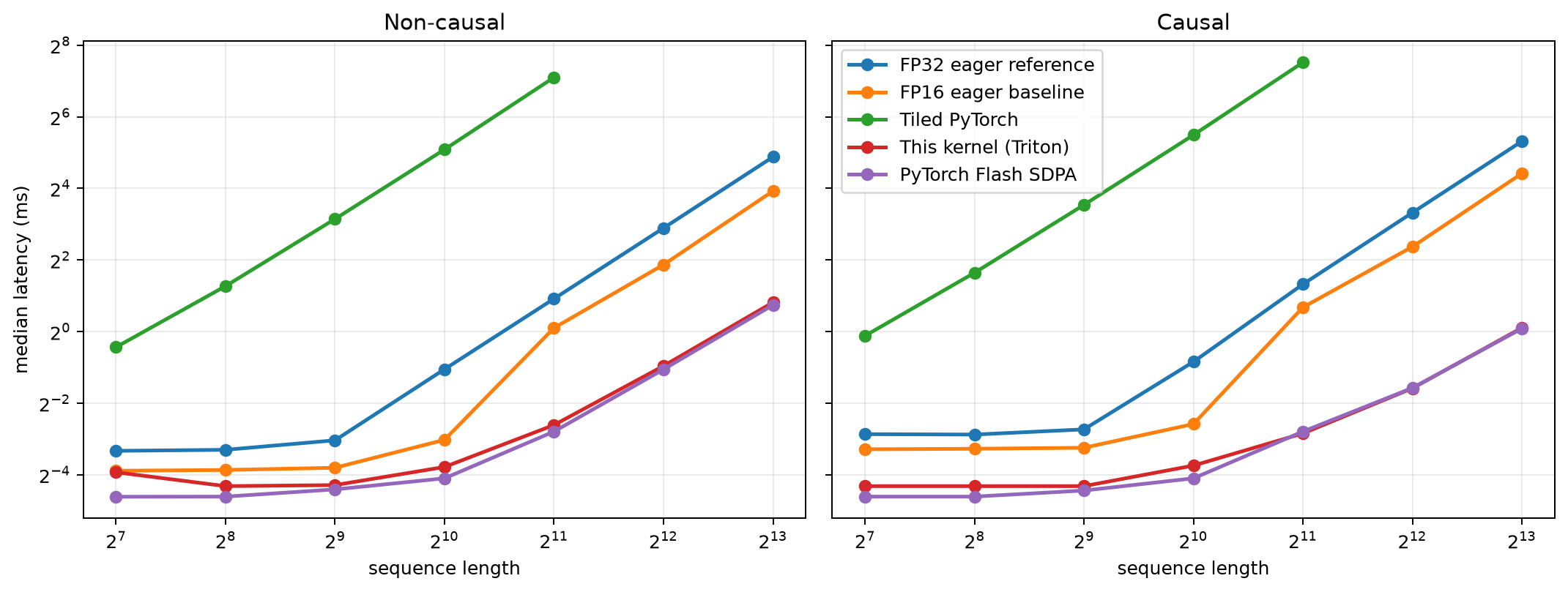
Measured latency: tiled PyTorch validates the algorithm but pays for Python loops and many small launches. The FP16 eager column removes the precision mismatch from the fusion comparison, and SDPA is explicitly constrained to its FlashAttention backend.
At N=8192:
- Non-causal Triton is
8.6×faster than FP16 eager and reaches95.1%of Flash SDPA throughput. - Causal Triton is
19.9×faster than FP16 eager and reaches98.7%of Flash SDPA throughput. - The causal kernel is faster here because it bounds the K/V loop by the current Q tile and skips the upper-right causal region.
The FP16 eager comparison keeps tensor precision aligned, although it still does
not isolate every implementation detail of the fused kernel. At N=1024, causal
Triton (0.075 ms) is close to non-causal Triton (0.073 ms)
despite skipping future tiles, consistent with fixed launch/tile costs dominating
at this short length.
Fusion alone does not guarantee a production-quality kernel. At N=128, fixed
costs are most visible and Triton reaches about 62% of Flash SDPA throughput in
the non-causal case. By N=8192, it reaches 95–99%, as avoiding full
score-matrix traffic becomes more important.
Useful throughput at N=8192 is 156.2 TFLOP/s non-causal and 127.7 TFLOP/s
causal for this Triton kernel. The numerator counts QK^T and PV only; the causal
number counts lower-triangular query/key pairs. These are algorithmic useful
FLOPs, not a hardware instruction count or percentage of theoretical peak.
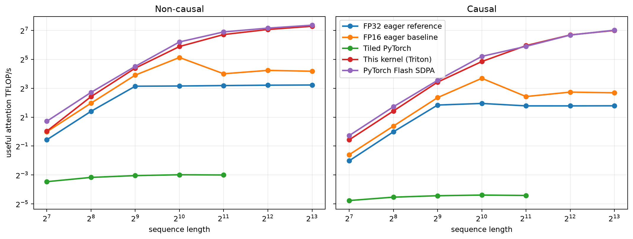
The trend of peak new GPU memory is more direct:
| N=8192 | FP32 eager ref | FP16 eager | This kernel (Triton) | Flash SDPA |
|---|---|---|---|---|
| non-causal | 8256 MiB | 4112 MiB | 16 MiB | 16.5 MiB |
| causal | 8320 MiB | 4176 MiB | 16 MiB | 16.5 MiB |
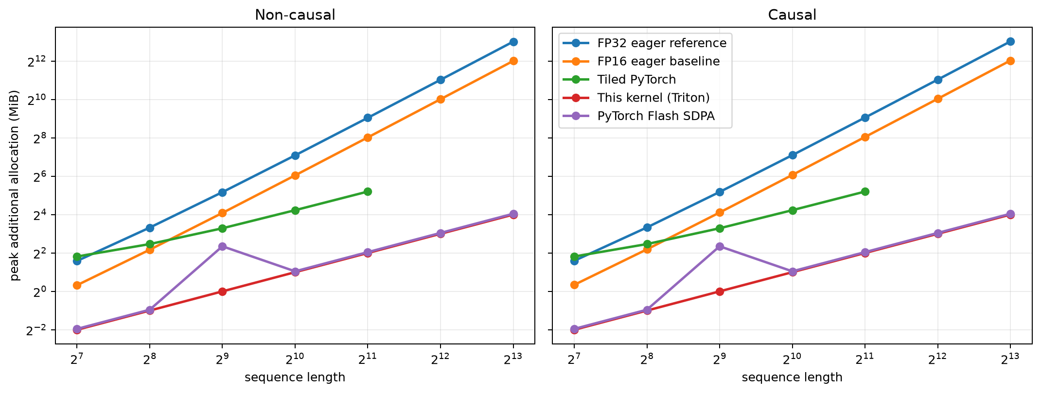
Measured incremental peak memory: eager FP32 scores and probabilities grow quadratically with sequence length; Triton and SDPA avoid those full intermediates.
The ratio 8320/16 = 520× is not a universal FlashAttention memory factor. The
eager reference deliberately computes FP32 scores, and the metric is incremental
peak allocation relative to the state immediately before each operator call.
The defensible conclusion is the scaling trend: eager materializes quadratic
intermediates, while the tested Triton and SDPA paths do not.
All 70 supplemental benchmark records are available in
results/supplemental/flash_attention_bench.csv,
with console output in
results/supplemental/benchmark.log.
The exact software/device record is in
environment.log.
The tables and plots report the recorded medians, not hand-picked best samples.
Profile Before Optimizing Further
A benchmark quantifies the gap but does not identify its cause. Profiling must connect Triton parameters to GPU resource use and hardware counters:
| Triton Choice | What You May Gain | What You May Pay |
|---|---|---|
Increase BLOCK_M/BLOCK_N |
More reuse and larger matrix operations | More registers and on-chip storage; occupancy may fall |
Increase num_warps |
More parallel threads within a single program | The number of programs that can reside simultaneously on each SM may be reduced |
Increase num_stages |
Load and compute have more pipeline overlap opportunities | Shared memory usage increases |
Useful metrics include DRAM throughput, Tensor Core utilization, achieved occupancy, register count, local-memory spills, and shared-memory use. If a larger tile increases latency, register pressure may have reduced occupancy or caused spills. Reading CUDA/CUTLASS/CuTe source at that point is no longer about recovering the algorithm; it is about instruction selection, data movement, and pipeline design.
Part 6: Back to vLLM—Same Recurrence, Different Data Layout
The implementation now has an evidence chain: online softmax makes tiled evaluation possible, Triton fuses the tiled loop, and tests cover correctness, latency, and incremental peak memory. It still cannot replace vLLM’s attention backend because its input organization and serving workload are much simpler.
Prefill and decode also stress different parts of the system. During
prefill, both Q_len and KV_len are large enough that avoiding a
materialized score matrix can deliver a direct benefit. The contiguous
self-attention implemented here resembles that workload. During decode,
Q_len is usually one or another small value, while the K/V history keeps
growing and may be physically paged. Paged addressing, GQA/MQA, split-KV, and
dynamic batching can matter more than the contiguous QK tiling shown here.
Understanding FlashAttention forward is therefore not the same as implementing
vLLM’s decode-attention path.
| Implementation in this article | Production vLLM inference path |
|---|---|
K/V is contiguous [B,H,N,D] |
KV cache is allocated in blocks/pages |
| Fixed-length self-attention | Mixed variable-length prefill/decode batch |
| Q, K, and V have the same length | Query and KV lengths vary by request and phase |
| Addresses follow tensor strides directly | block_table maps logical blocks to physical blocks |
| MHA | Also supports MQA/GQA |
| One program scans the K/V range | Long K/V ranges may use split-KV and a combine step |
| Fixed M/N tiles and warp count | Tuning varies by GPU, dtype, and head size |
| Forward only | Production code covers broader masks, dtypes, and interface contracts |
The paged-KV path in the previous article can be rewritten as:
This kernel (Triton)
Q tile + contiguous K/V tiles
    + online softmax

vLLM FlashAttention backend
    Q tile + varlen metadata
+ block_table paging addressing
    + paged K/V tiles
    + online softmax
    + split-KV / backend dispatch
The main new dimension is indirect addressing. This article finds the jth K/V
tile with a contiguous stride. vLLM first consults block_table, translates
logical KV positions into physical cache blocks, and then loads the data. A page
is a storage/allocation unit; a tile is a computation unit. Their boundaries
need not coincide.
Part 2 reads the production paged-KV path; Part 3 implements the core recurrence over contiguous tensors. The two views answer different questions: how vLLM addresses serving-time K/V state, and how online softmax becomes a fused kernel. The production templates and hardware branches remain complex, but their data flow is now easier to locate in code.
The Full Progression in One Diagram
Explicit PyTorch attention
Full scores/probabilities spill to HBM
↓ Rewrite softmax with m/l/acc
Tiled PyTorch
The math is correct, but Python loops trigger many kernel launches
↓ Put the K/V loop and recurrence into the same program
Triton kernel
The current scores tile remains on-chip and only the final output is written
↓ Bounds / accuracy / memory / latency validation
Back to vLLM
The recurrence remains; production adds varlen, paged KV, and backend scheduling
Each step solves one problem. Explicit PyTorch provides a trusted reference; online softmax makes exact tiling possible; Triton removes repeated launches and intermediate write-backs; validation checks that speed did not hide a boundary or numerical error; and the final comparison separates this contiguous prefill kernel from vLLM’s production serving path.
Putting the three articles together, we have started with:
llm.generate
  -> EngineCore / Scheduler
  -> packed input / paged-KV metadata
  -> reshape_and_cache_flash
  -> paged FlashAttention data flow
  -> contiguous-attention Triton forward kernel
The three-part series now reaches from Python scheduling to an executable
attention kernel. A useful next step toward production is not to copy one
generation of FlashAttention line by line, but to add variable-length inputs
and block_table addressing to this kernel, then observe how paged addressing
changes program mapping, tile loads, and the performance bottleneck.
How This Implementation Relates to FlashAttention Versions
This article focuses on the algorithmic structure shared across generations; it does not reproduce any one release line by line:
- FlashAttention v1 establishes IO-aware tiling, online softmax, and
recomputation in backward. It retains exact attention’s
O(N²D)arithmetic while reducing HBM traffic and auxiliary storage. - FlashAttention-2 further reduces non-matrix multiplication FLOPs, increases thread-block parallelism within a single head, and repartitions warp work to reduce shared-memory communication.
- FlashAttention-3 targets Hopper and uses asynchronous execution, warp specialization, TMA, and WGMMA in its pipeline.
- FlashAttention-4: As of September 3, 2026, the official repository exposes a
FlashAttention-4 (CuTeDSL) implementation for Hopper and Blackwell, while
PyPI still labels its latest
4.0.0b29build as a pre-release. Hardware coverage, interfaces, and maturity may change; consult the current repository and package metadata. The learning path therefore need not end specifically in handwritten CUDA/CUTLASS.
Those differences deserve a separate article. Here the important invariant is
Q tile → scan K/V tiles → online softmax → output accumulator; each generation
maps that structure onto different hardware and work-partitioning strategies.
What this article doesn’t cover
- Backward propagation and recomputation; the vLLM inference path only requires the forward pass implemented here.
- Dropout, attention bias, arbitrary masks, and cross-attention.
- GQA/MQA, variable-length inputs, paged KV, and split-KV combination.
- Autotuning, Tensor Core instruction selection, and shared-memory bank conflicts.
- Hardware-counter attribution and a careful percent-of-peak analysis. The current report measures latency and memory but does not claim a cause for the remaining SDPA gap.
- Warp specialization, asynchronous pipelining and hardware trade-offs implemented in each generation of FlashAttention.
- Beating production FlashAttention is not a goal. PyTorch SDPA is used as a framework baseline; the original run did not record its selected backend.
References and Companion Artifacts
- Source code and complete reproduction package: PyTorch reference, tiled online softmax, Triton kernel, validation scripts, and run instructions.
- Supplemental correctness log: All 71 cases passed.
-
Supplemental benchmark log and full CSV data: 70 performance records in total.
- FlashAttention original paper: FlashAttention: Fast and Memory-Efficient Exact Attention with IO-Awareness.
- FlashAttention-2 Paper: Reduce non-matrix multiplication overhead and improve thread-block/warp work partitioning.
- FlashAttention-4 paper: algorithm and kernel-pipelining co-design for asymmetric hardware scaling.
- Official FlashAttention repository: implementations across generations and the current FlashAttention-4 description.
- FlashAttention-4 PyPI Page: Used to check the
4.0.0b*pre-release version and current release status. - Triton official tutorial: Vector Add, Fused Softmax, Matrix Multiplication, Fused Attention.
- Triton programming model and language API: blocked programs and operations such as
program_id,arange, anddot. - PyTorch
scaled_dot_product_attentionDocumentation: Used to illustrate that SDPA automatically selects different implementations. - Complete code:
flash_attention_lab.py. - Drawing code:
plot_results.py. - Run instructions:
README.md. - Figure sources: Excalidraw files
assets/figC0throughfigC4.
The implementation is deliberately compact so its data flow can be inspected. All measurement figures come from the stated RTX 4090 Linux environment; the correctness log, benchmark CSV, plotting script, and environment versions are published for review and reproduction.